Stochastic Local Search Computer Science cpsc 322 Lecture

Stochastic Local Search Computer Science cpsc 322, Lecture 15 (Textbook Chpt 4. 8) May, 30, 2017 CPSC 322, Lecture 15 Slide 1

Lecture Overview • Recap Local Search in CSPs • Stochastic Local Search (SLS) • Comparing SLS algorithms CPSC 322, Lecture 15 Slide 2

Local Search: Summary • A useful method in practice for large CSPs • Start from a possible world • Generate some neighbors ( “similar” possible worlds) • Move from current node to a neighbor, selected to minimize/maximize a scoring function which combines: ü Info about how many constraints are violated/satisfied ü Information about the cost/quality of the solution (you want the best solution, not just a solution) CPSC 322, Lecture 15 Slide 3

CPSC 322, Lecture 15 Slide 4

Hill Climbing NOTE: Everything that will be said for Hill Climbing is also true for Greedy Descent CPSC 322, Lecture 5 Slide 5

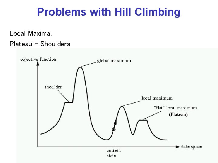
Problems with Hill Climbing Local Maxima. Plateau - Shoulders (Plateau) CPSC 322, Lecture 5 Slide 6

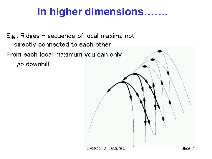
In higher dimensions……. E. g. , Ridges – sequence of local maxima not directly connected to each other From each local maximum you can only go downhill CPSC 322, Lecture 5 Slide 7

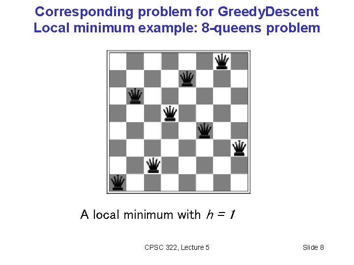
Corresponding problem for Greedy. Descent Local minimum example: 8 -queens problem A local minimum with h = 1 CPSC 322, Lecture 5 Slide 8

Lecture Overview • Recap Local Search in CSPs • Stochastic Local Search (SLS) • Comparing SLS algorithms CPSC 322, Lecture 15 Slide 9

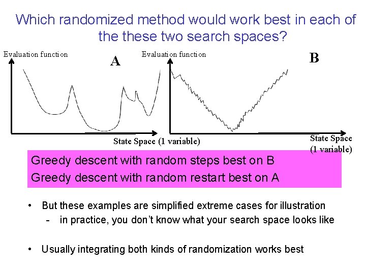
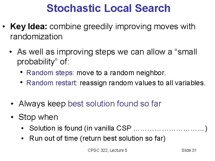
Stochastic Local Search GOAL: We want our local search • to be guided by the scoring function • Not to get stuck in local maxima/minima, plateaus etc. • SOLUTION: We can alternate a) Hill-climbing steps b) Random steps: move to a random neighbor. c) Random restart: reassign random values to all variables. CPSC 322, Lecture 15 Slide 10

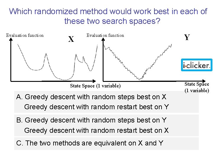
Which randomized method would work best in each of these two search spaces? Evaluation function X Evaluation function State Space (1 variable) A. Greedy descent with random steps best on X Greedy descent with random restart best on Y B. Greedy descent with random steps best on Y Greedy descent with random restart best on X C. The two methods are equivalent on X and Y Y State Space (1 variable)

Which randomized method would work best in each of these two search spaces? Evaluation function A Evaluation function State Space (1 variable) Greedy descent with random steps best on B Greedy descent with random restart best on A B State Space (1 variable) • But these examples are simplified extreme cases for illustration - in practice, you don’t know what your search space looks like • Usually integrating both kinds of randomization works best

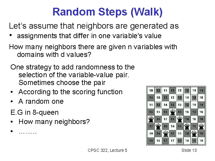
Random Steps (Walk) Let’s assume that neighbors are generated as • assignments that differ in one variable's value How many neighbors there are given n variables with domains with d values? One strategy to add randomness to the selection of the variable-value pair. Sometimes choose the pair • According to the scoring function • A random one E. G in 8 -queen • How many neighbors? • ……. . CPSC 322, Lecture 5 Slide 13

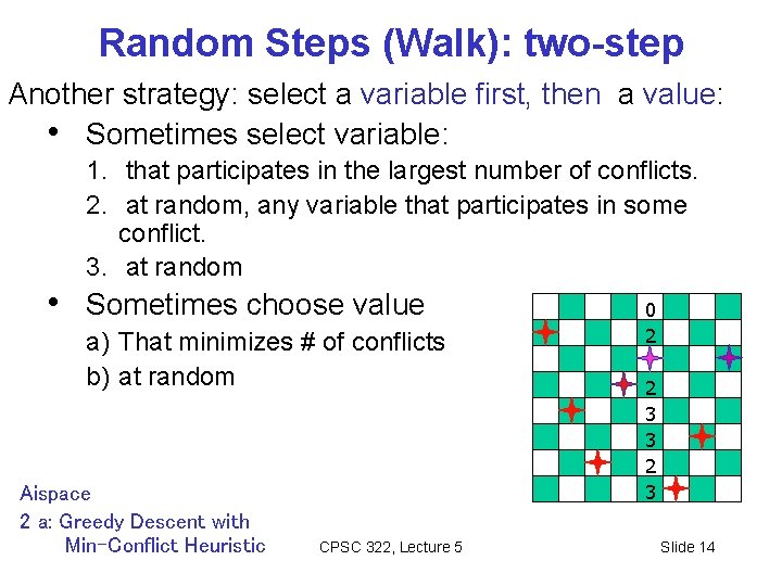
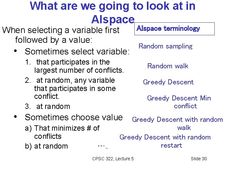
Random Steps (Walk): two-step Another strategy: select a variable first, then a value: • Sometimes select variable: 1. that participates in the largest number of conflicts. 2. at random, any variable that participates in some conflict. 3. at random • Sometimes choose value a) That minimizes # of conflicts b) at random Aispace 2 a: Greedy Descent with Min-Conflict Heuristic CPSC 322, Lecture 5 0 2 2 3 3 2 3 Slide 14

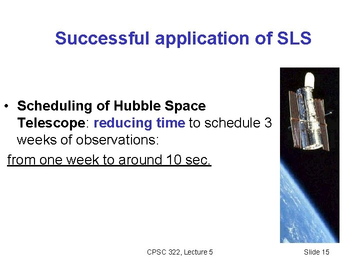
Successful application of SLS • Scheduling of Hubble Space Telescope: reducing time to schedule 3 weeks of observations: from one week to around 10 sec. CPSC 322, Lecture 5 Slide 15

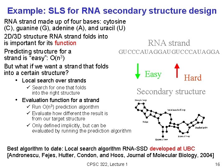
Example: SLS for RNA secondary structure design RNA strand made up of four bases: cytosine (C), guanine (G), adenine (A), and uracil (U) 2 D/3 D structure RNA strand folds into is important for its function RNA strand Predicting structure for a GUCCCAUAGGAUGUCCCAUAGGA 3 strand is “easy”: O(n ) But what if we want a strand that folds into a certain structure? Easy Hard • Local search over strands ü Search for one that folds into the right structure • Evaluation function for a strand Secondary structure ü Run O(n 3) prediction algorithm ü Evaluate how different the result is from our target structure ü Only defined implicitly, but can be evaluated by running the prediction algorithm Best algorithm to date: Local search algorithm RNA-SSD developed at UBC [Andronescu, Fejes, Hutter, Condon, and Hoos, Journal of Molecular Biology, 2004] CPSC 322, Lecture 1 16

CSP/logic: formal verification Hardware verification (e. g. , IBM) Software verification (small to medium programs) Most progress in the last 10 years based on: Encodings into propositional satisfiability (SAT) CPSC 322, Lecture 1 17

(Stochastic) Local search advantage: Online setting • When the problem can change (particularly important in scheduling) • E. g. , schedule for airline: thousands of flights and thousands of personnel assignment • Storm can render the schedule infeasible • Goal: Repair with minimum number of changes • This can be easily done with a local search starting form the current schedule • Other techniques usually: • require more time • might find solution requiring many 5 more changes CPSC 322, Lecture Slide 18

SLS limitations • Typically no guarantee to find a solution even if one exists • SLS algorithms can sometimes stagnate ü Get caught in one region of the search space and never terminate • Very hard to analyze theoretically • Not able to show that no solution exists • SLS simply won’t terminate • You don’t know whether the problem is infeasible or the algorithm has stagnated

SLS Advantage: anytime algorithms • When should the algorithm be stopped ? • When a solution is found • • (e. g. no constraint violations) Or when we are out of time: you have to act NOW Anytime algorithm: ü maintain the node with best h found so far (the “incumbent”) ü given more time, can improve its incumbent

Lecture Overview • Recap Local Search in CSPs • Stochastic Local Search (SLS) • Comparing SLS algorithms CPSC 322, Lecture 15 Slide 21

Evaluating SLS algorithms • SLS algorithms are randomized • The time taken until they solve a problem is a random variable • It is entirely normal to have runtime variations of 2 orders of magnitude in repeated runs! ü E. g. 0. 1 seconds in one run, 10 seconds in the next one ü On the same problem instance (only difference: random seed) ü Sometimes SLS algorithm doesn’t even terminate at all: stagnation • If an SLS algorithm sometimes stagnates, what is its mean runtime (across many runs)? • Infinity! • In practice, one often counts timeouts as some fixed large value X • Still, summary statistics, such as mean run time or median run time, don't tell the whole story ü E. g. would penalize an algorithm that often finds a solution quickly but sometime stagnates

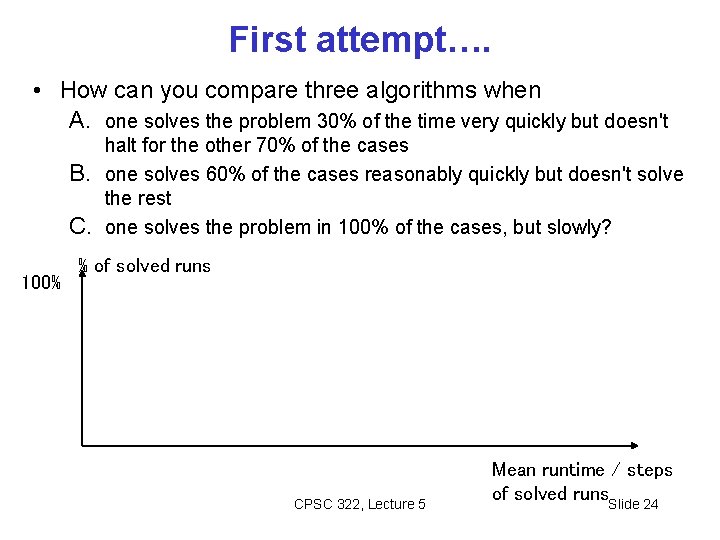
First attempt…. • How can you compare three algorithms when A. one solves the problem 30% of the time very quickly but doesn't B. C. 100% halt for the other 70% of the cases one solves 60% of the cases reasonably quickly but doesn't solve the rest one solves the problem in 100% of the cases, but slowly? % of solved runs CPSC 322, Lecture 5 Mean runtime / steps of solved runs. Slide 24

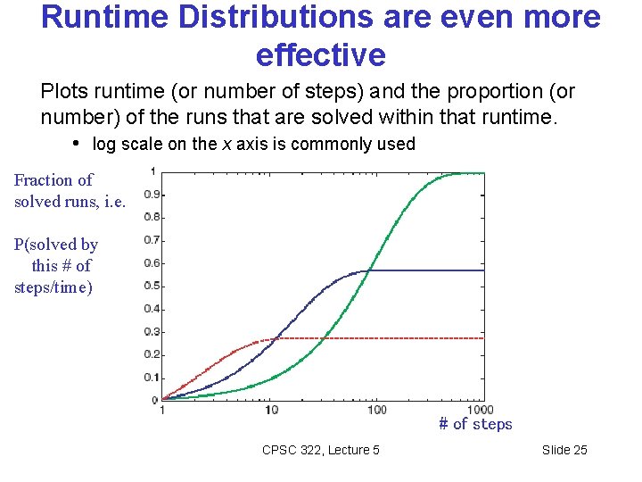
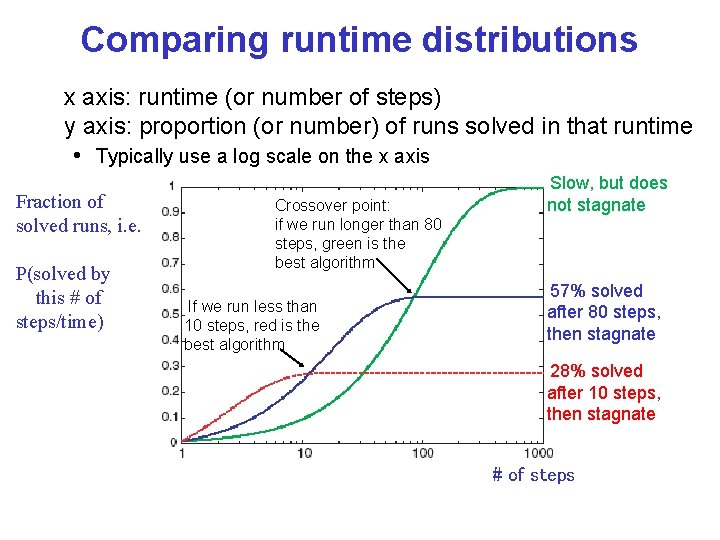
Runtime Distributions are even more effective Plots runtime (or number of steps) and the proportion (or number) of the runs that are solved within that runtime. • log scale on the x axis is commonly used Fraction of solved runs, i. e. P(solved by this # of steps/time) # of steps CPSC 322, Lecture 5 Slide 25

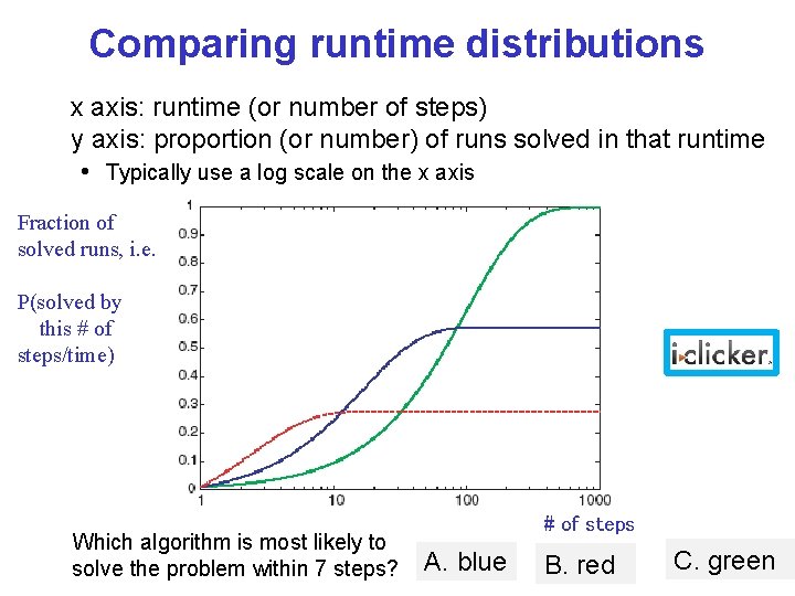
Comparing runtime distributions x axis: runtime (or number of steps) y axis: proportion (or number) of runs solved in that runtime • Typically use a log scale on the x axis Fraction of solved runs, i. e. P(solved by this # of steps/time) Which algorithm is most likely to solve the problem within 7 steps? # of steps A. blue B. red C. green

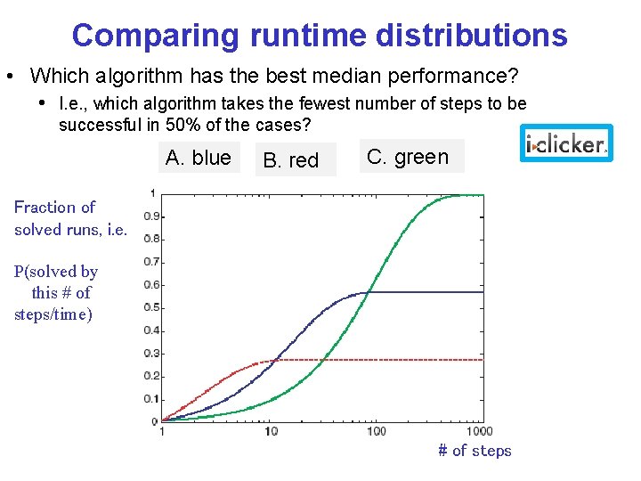
Comparing runtime distributions • Which algorithm has the best median performance? • I. e. , which algorithm takes the fewest number of steps to be successful in 50% of the cases? A. blue B. red C. green Fraction of solved runs, i. e. P(solved by this # of steps/time) # of steps

Comparing runtime distributions x axis: runtime (or number of steps) y axis: proportion (or number) of runs solved in that runtime • Typically use a log scale on the x axis Fraction of solved runs, i. e. P(solved by this # of steps/time) Crossover point: if we run longer than 80 steps, green is the best algorithm If we run less than 10 steps, red is the best algorithm Slow, but does not stagnate 57% solved after 80 steps, then stagnate 28% solved after 10 steps, then stagnate # of steps

Runtime distributions in AIspace • Let’s look at some algorithms and their runtime distributions: 1. Greedy Descent 2. Random Sampling 3. Random Walk 4. Greedy Descent with random walk • Simple scheduling problem 2 in AIspace:

What are we going to look at in AIspace terminology When selecting a variable first followed by a value: Random sampling • Sometimes select variable: 1. that participates in the largest number of conflicts. 2. at random, any variable that participates in some conflict. 3. at random Random walk Greedy Descent Min conflict • Sometimes choose value a) That minimizes # of conflicts …. . b) at random Greedy Descent with random walk Greedy Descent with random restart CPSC 322, Lecture 5 Slide 30

Stochastic Local Search • Key Idea: combine greedily improving moves with randomization • As well as improving steps we can allow a “small probability” of: • Random steps: move to a random neighbor. • Random restart: reassign random values to all variables. • Always keep best solution found so far • Stop when • Solution is found (in vanilla CSP ……………) • Run out of time (return best solution so far) CPSC 322, Lecture 5 Slide 31

Learning Goals for today’s class You can: • Implement SLS with • random steps (1 -step, 2 -step versions) • random restart • Compare SLS algorithms with runtime distributions CPSC 322, Lecture 4 Slide 32

Assign-2 • Will be out today – due June Next Class • Finish CSPs: More SLS variants Chp 4. 9 • Planning: Representations and Forward Search Chp 8. 1 - 8. 2 • Planning: Heuristics and CSP Planning Chp 8. 4 CPSC 322, Lecture 15 Slide 33