Stochastic Local Search CPSC 322 CSP 6 Textbook

Stochastic Local Search CPSC 322 – CSP 6 Textbook § 4. 8 February 9, 2011

Lecture Overview • Recap: local search • Stochastic local search (SLS) • Comparing SLS algorithms • Pros and cons of SLS • Time-permitting: Types of SLS algorithms 2

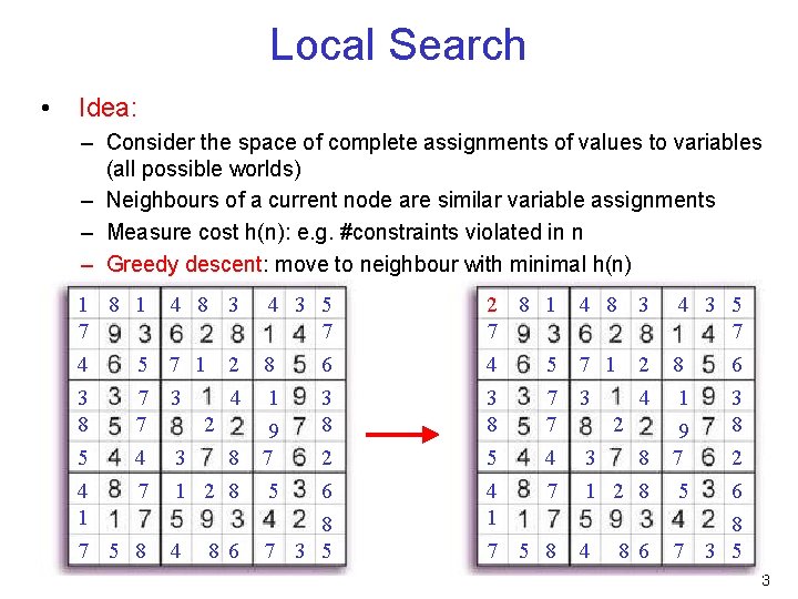
Local Search • Idea: – Consider the space of complete assignments of values to variables (all possible worlds) – Neighbours of a current node are similar variable assignments – Measure cost h(n): e. g. #constraints violated in n – Greedy descent: move to neighbour with minimal h(n) 1 8 1 4 7 4 5 7 3 8 7 5 4 3 4 7 1 1 7 5 8 4 8 3 4 3 5 7 1 2 8 6 4 1 3 2 8 9 8 7 2 2 8 5 6 8 8 6 7 3 5 2 8 1 4 7 4 5 7 3 8 7 5 4 3 4 7 1 1 7 5 8 4 8 3 4 3 5 7 1 2 8 6 4 1 3 2 8 9 8 7 2 2 8 5 6 8 8 6 7 3 5 3

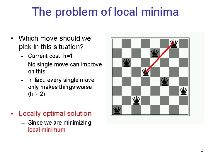
The problem of local minima • Which move should we pick in this situation? - Current cost: h=1 - No single move can improve on this - In fact, every single move only makes things worse (h 2) • Locally optimal solution – Since we are minimizing: local minimum 4

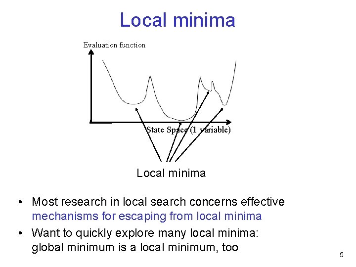
Local minima Evaluation function State Space (1 variable) Local minima • Most research in local search concerns effective mechanisms for escaping from local minima • Want to quickly explore many local minima: global minimum is a local minimum, too 5

Lecture Overview • Recap: local search • Stochastic local search (SLS) • Comparing SLS algorithms • Pros and cons of SLS • Time-permitting: Types of SLS algorithms 6

Stochastic Local Search • We will use greedy steps to find local minima • We will use randomness to avoid getting trapped in local minima 7

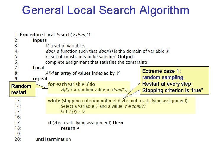
General Local Search Algorithm Random restart Extreme case 1: random sampling. Restart at every step: Stopping criterion is “true”

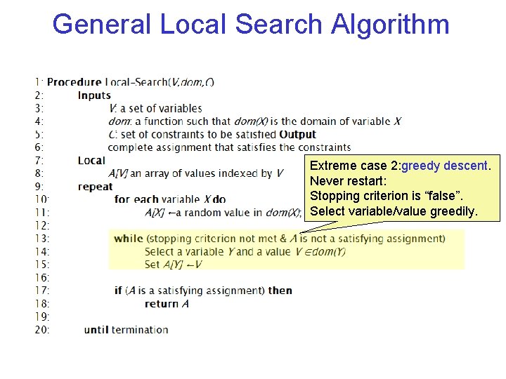
General Local Search Algorithm Extreme case 2: greedy descent. Never restart: Stopping criterion is “false”. Select variable/value greedily.

Tracing SLS algorithms in AIspace • Let’s look at these algorithms in AIspace: - Greedy Descent - Random Sampling • Simple scheduling problem 2 in AIspace: 10

Greedy descent vs. Random sampling • Greedy descent is – good for finding local minima – bad for exploring new parts of the search space • Random sampling is – good for exploring new parts of the search space – bad for finding local minima • A mix of the two can work very well 11

Greedy Descent + Randomness • Greedy steps – Move to neighbour with best evaluation function value • Next to greedy steps, we can allow for: 1. Random restart: reassign random values to all variables (i. e. start fresh) 2. Random steps: move to a random neighbour • Only doing random steps (no greedy steps at all) is called “random walk” 12

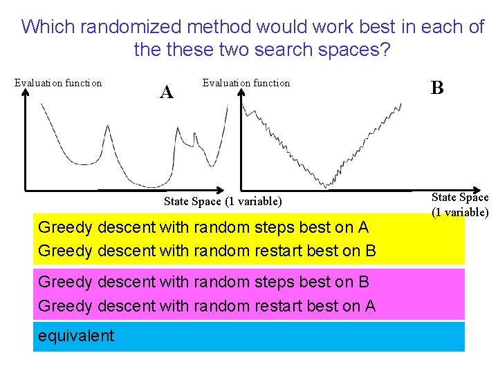
Which randomized method would work best in each of these two search spaces? Evaluation function A Evaluation function State Space (1 variable) Greedy descent with random steps best on A Greedy descent with random restart best on B Greedy descent with random steps best on B Greedy descent with random restart best on A equivalent B State Space (1 variable)

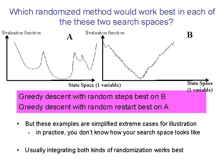
Which randomized method would work best in each of these two search spaces? Evaluation function A Evaluation function State Space (1 variable) Greedy descent with random steps best on B Greedy descent with random restart best on A B State Space (1 variable) • But these examples are simplified extreme cases for illustration - in practice, you don’t know how your search space looks like • Usually integrating both kinds of randomization works best

Stochastic Local Search for CSPs • More examples of ways to add randomness to local search for a CSP • In one stage selection of variable and value: – instead choose a random variable-value pair • In two stage selection (first select variable V, then new value for V): – Selecting variables: • Sometimes choose the variable which participates in the largest number of conflicts • Sometimes choose a random variable that participates in some conflict • Sometimes choose a random variable – Selecting values • Sometimes choose the best value for the chosen variable: the one yielding minimal h(n) • Sometimes choose a random value for the chosen variable 15

Greedy Descent with Min-Conflict Heuristic • One of the best SLS techniques for CSP solving: – At random, select one of the variables v that participates in a violated constraint – Set v to one of the values that minimizes the number of unsatisfied constraints • Can be implemented efficiently: – Data structure 1 stores currently violated constraints – Data structure 2 stores variables that are involved in violated constraints – Each step only yields incremental changes to these data structures • Most SLS algorithms can be implemented similarly efficiently very small complexity per search step 16

Lecture Overview • Recap: local search • Stochastic local search (SLS) • Comparing SLS algorithms • Pros and cons of SLS • Time-permitting: Types of SLS algorithms 17

Evaluating SLS algorithms • SLS algorithms are randomized – The time taken until they solve a problem is a random variable – It is entirely normal to have runtime variations of 2 orders of magnitude in repeated runs! • E. g. 0. 1 seconds in one run, 10 seconds in the next one • On the same problem instance (only difference: random seed) • Sometimes SLS algorithm doesn’t even terminate at all: stagnation • If an SLS algorithm sometimes stagnates, what is its mean runtime (across many runs)? – Infinity! – In practice, one often counts timeouts as some fixed large value X • But results depend on which X is chosen 18

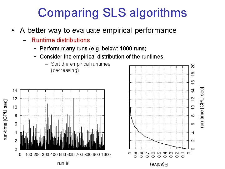
Comparing SLS algorithms • A better way to evaluate empirical performance – Runtime distributions • Perform many runs (e. g. below: 1000 runs) • Consider the empirical distribution of the runtimes – Sort the empirical runtimes (decreasing) 19

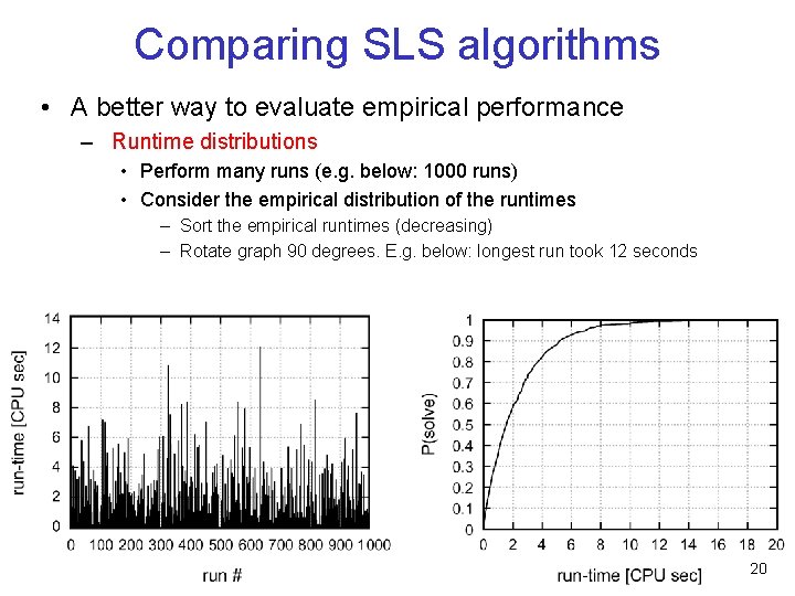
Comparing SLS algorithms • A better way to evaluate empirical performance – Runtime distributions • Perform many runs (e. g. below: 1000 runs) • Consider the empirical distribution of the runtimes – Sort the empirical runtimes (decreasing) – Rotate graph 90 degrees. E. g. below: longest run took 12 seconds 20

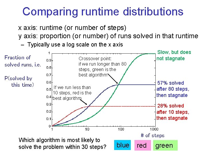
Comparing runtime distributions x axis: runtime (or number of steps) y axis: proportion (or number) of runs solved in that runtime – Typically use a log scale on the x axis Fraction of solved runs, i. e. P(solved by this time) Slow, but does not stagnate Crossover point: if we run longer than 80 steps, green is the best algorithm 57% solved after 80 steps, then stagnate If we run less than 10 steps, red is the best algorithm 28% solved after 10 steps, then stagnate Which algorithm is most likely to solve the problem within 30 steps? # of steps blue red green

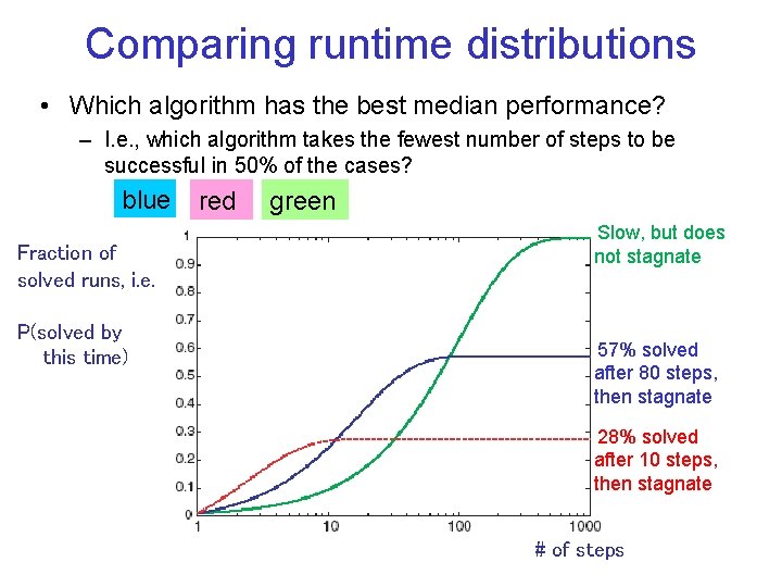
Comparing runtime distributions • Which algorithm has the best median performance? – I. e. , which algorithm takes the fewest number of steps to be successful in 50% of the cases? blue Fraction of solved runs, i. e. P(solved by this time) red green Slow, but does not stagnate 57% solved after 80 steps, then stagnate 28% solved after 10 steps, then stagnate # of steps

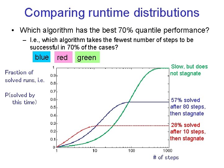
Comparing runtime distributions • Which algorithm has the best 70% quantile performance? – I. e. , which algorithm takes the fewest number of steps to be successful in 70% of the cases? blue Fraction of solved runs, i. e. P(solved by this time) red green Slow, but does not stagnate 57% solved after 80 steps, then stagnate 28% solved after 10 steps, then stagnate # of steps

Runtime distributions in AIspace • Let’s look at some algorithms and their runtime distributions: - Greedy Descent Random Sampling Random Walk Greedy Descent with random walk • Simple scheduling problem 2 in AIspace: 24

Lecture Overview • Recap: local search • Stochastic local search (SLS) • Comparing SLS algorithms • Pros and cons of SLS • Time-permitting: Types of SLS algorithms 25

SLS limitations • Typically no guarantee to find a solution even if one exists – SLS algorithms can sometimes stagnate – Get caught in one region of the search space and never terminate – Very hard to analyze theoretically • Not able to show that no solution exists – SLS simply won’t terminate – You don’t know whether the problem is infeasible or the algorithm stagnates • When do you stop? ? – When you know the solution found is optimal (e. g. no more constraint violations) – Or when you’re out of time: we have to act NOW – Anytime algorithm: • maintain the node with best h found so far (the “incumbent”) • given more time, can improve its incumbent 26

SLS generality: Constraint Optimization Problems • Constraint Satisfaction Problems – Hard constraints: need to satisfy all of them – All models are equally good • Constraint Optimization Problems – Hard constraints: need to satisfy all of them – Soft constraints: need to satisfy them as good as possible – Can have weighted constraints • Minimize h(n) = sum of weights of constraints unsatisfied in n • Hard constraints have a very large weight • Some soft constraints can be more important than other soft constraints larger weight – All local search methods we will discuss work just as well for constraint optimization • all they need is an evaluation function h 27

Example for constraint optimization problem Exam scheduling – Hard constraints: • Cannot have an exam in too small a room • Cannot have multiple exams in the same room in the same time slot • … – Soft constraints • • Student should really not have to write two exams at the same time Students should not have multiple exams on the same day It would be nice if students have their exams spread out … Programming question “SLS for scheduling” in assignment 2 – Limited version of the real world problem 28

SLS generality: optimization of arbitrary functions • SLS is even more general – SLS’s generality doesn’t stop at constraint optimization – We can optimize arbitrary functions f(x 1, …, xn) that we can evaluate for any complete assignment of their n inputs – The function’s inputs correspond to our possible worlds, i. e. to the SLS search states • Example: RNA secondary structure design 29

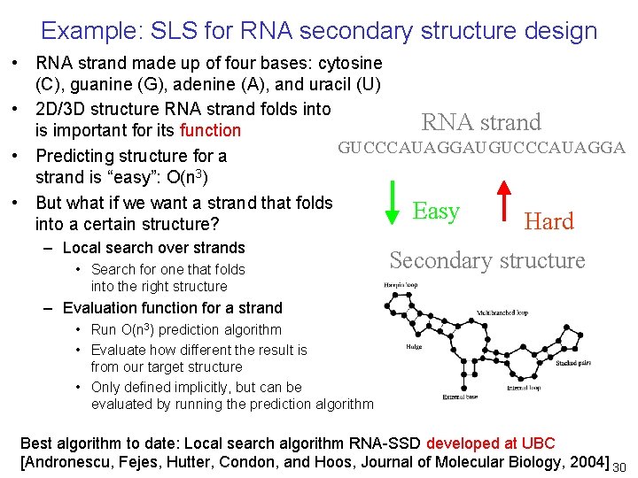
Example: SLS for RNA secondary structure design • RNA strand made up of four bases: cytosine (C), guanine (G), adenine (A), and uracil (U) • 2 D/3 D structure RNA strand folds into RNA strand is important for its function GUCCCAUAGGAUGUCCCAUAGGA • Predicting structure for a strand is “easy”: O(n 3) • But what if we want a strand that folds Easy Hard into a certain structure? – Local search over strands • Search for one that folds into the right structure Secondary structure – Evaluation function for a strand • Run O(n 3) prediction algorithm • Evaluate how different the result is from our target structure • Only defined implicitly, but can be evaluated by running the prediction algorithm Best algorithm to date: Local search algorithm RNA-SSD developed at UBC [Andronescu, Fejes, Hutter, Condon, and Hoos, Journal of Molecular Biology, 2004] 30

SLS generality: dynamically changing problems • The problem may change over time – Particularly important in scheduling – E. g. , schedule for airline: • Thousands of flights and thousands of personnel assignments • A storm can render the schedule infeasible • Goal: Repair the schedule with minimum number of changes – Often easy for SLS starting form the current schedule – Other techniques usually: • Require more time • Might find solution requiring many more changes 31

Lecture Overview • Recap: local search • Stochastic local search (SLS) • Comparing SLS algorithms • Pros and cons of SLS • Time-permitting: Types of SLS algorithms 32

Many different types of local search • We will only touch on each of them very briefly • Only need to know them on a high level • You will have to choose and implement one of them for programming assignment “SLS for scheduling” 33

Simulated Annealing • Annealing: a metallurgical process where metals are hardened by being slowly cooled • Analogy: – start with a high “temperature": high tendency to take random steps – Over time, cool down: only take random steps that are not too bad • Details: – At node n, select a random neighbour n’ – If h(n’) < h(n), move to n’ (i. e. accept all improving steps) – Otherwise, adopt it with a probability depending on • How much worse n’ is then n • the current temperature T: high T tends to accept even very bad moves • Probability of accepting worsening move: exp ( (h(n) – h(n’) / T ) – Temperature reduces over time, according to an annealing schedule • “Finding a good annealing schedule is an art” • E. g. geometric cooling: every step multiply T by some constant < 1 34

Tabu Search • Mark partial assignments as tabu (taboo) – Prevents repeatedly visiting the same (or similar) local minima – Maintain a queue of k variable/value pairs that are taboo – E. g. , when changing a variable V’s value from 2 to 4, we cannot change it back to 2 for the next k steps – k is a parameter that needs to be optimized empirically 35

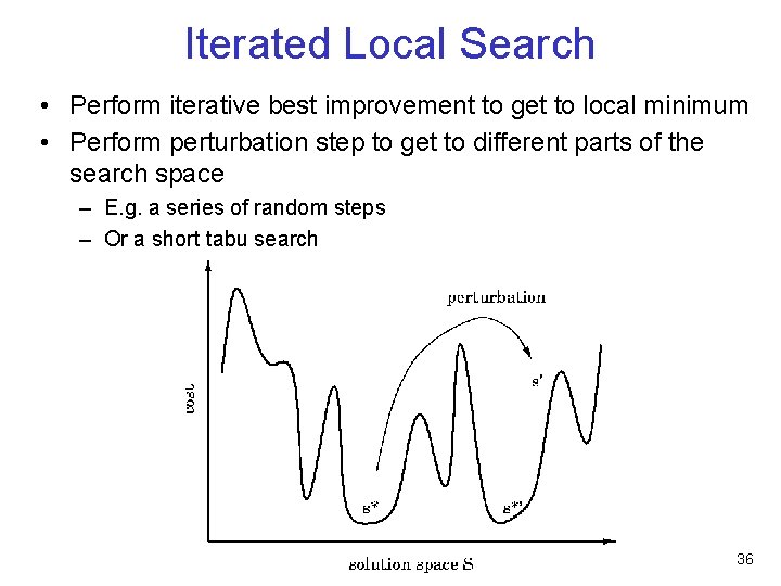
Iterated Local Search • Perform iterative best improvement to get to local minimum • Perform perturbation step to get to different parts of the search space – E. g. a series of random steps – Or a short tabu search 36

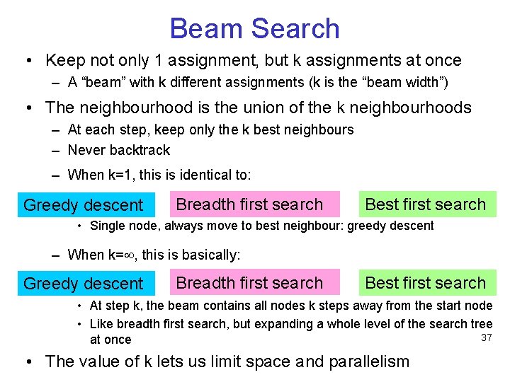
Beam Search • Keep not only 1 assignment, but k assignments at once – A “beam” with k different assignments (k is the “beam width”) • The neighbourhood is the union of the k neighbourhoods – At each step, keep only the k best neighbours – Never backtrack – When k=1, this is identical to: Greedy descent Breadth first search Best first search • Single node, always move to best neighbour: greedy descent – When k= , this is basically: Greedy descent Breadth first search Best first search • At step k, the beam contains all nodes k steps away from the start node • Like breadth first search, but expanding a whole level of the search tree 37 at once • The value of k lets us limit space and parallelism

Stochastic Beam Search • Like beam search, but you probabilistically choose the k nodes at the next step (“generation”) • The probability that a neighbour is chosen is proportional to the value of the evaluation function – This maintains diversity amongst the nodes – The scoring function value reflects the fitness of the node • Biological metaphor: – like asexual reproduction: each node gives its mutations and the fittest ones survive 38

Genetic Algorithms • Like stochastic beam search, but pairs of nodes are combined to create the offspring • For each generation: – Randomly choose pairs of nodes (“parents”), with the best-scoring nodes being more likely to be chosen • For each pair, perform a cross-over: create two offspring each taking different parts of their parents – Mutate some values for each offspring 39

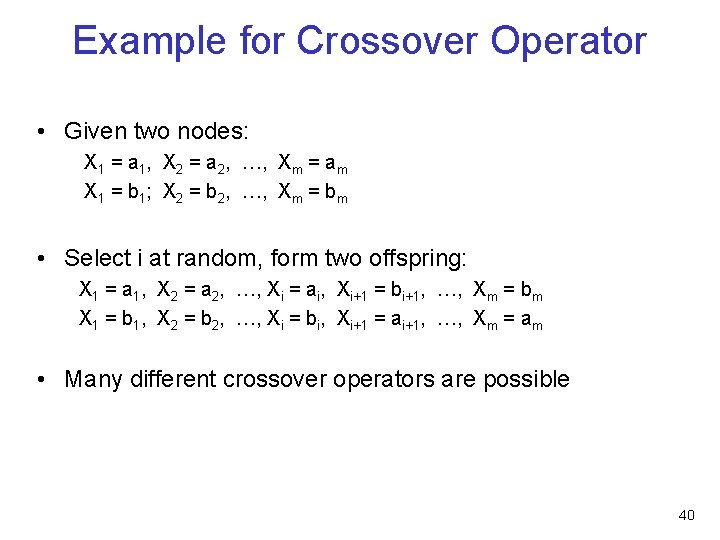
Example for Crossover Operator • Given two nodes: X 1 = a 1, X 2 = a 2, …, Xm = am X 1 = b 1; X 2 = b 2, …, Xm = bm • Select i at random, form two offspring: X 1 = a 1, X 2 = a 2, …, Xi = ai, Xi+1 = bi+1, …, Xm = bm X 1 = b 1, X 2 = b 2, …, Xi = bi, Xi+1 = ai+1, …, Xm = am • Many different crossover operators are possible 40

Local Search Learning Goals • Implement local search for a CSP. – Implement different ways to generate neighbors – Implement scoring functions to solve a CSP by local search through either greedy descent or hill-climbing. • Implement SLS with – random steps (1 -step, 2 -step versions) – random restart • Compare SLS algorithms with runtime distributions • Coming up: – Assignment #2 is available on Web. CT (due Wednesday, Feb 23 rd) – Next class: finish local search; then move to planning (Chapter 8)