Statistical Thermodynamics Lecture 19 Free Energies in Modern

Statistical Thermodynamics Lecture 19: Free Energies in Modern Computational Statistical Thermodynamics: WHAM and Related Methods Dr. Ronald M. Levy ronlevy@temple. edu

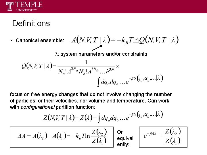
Definitions • Canonical ensemble: l: system parameters and/or constraints focus on free energy changes that do not involve changing the number of particles, or their velocities, nor volume and temperature. Can work with configurational partition function: Or equival ently:

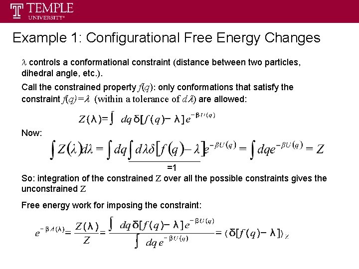
Example 1: Configurational Free Energy Changes l controls a conformational constraint (distance between two particles, dihedral angle, etc. ). Call the constrained property f(q): only conformations that satisfy the constraint f(q)=l (within a tolerance of dl) are allowed: Now: =1 So: integration of the constrained Z over all the possible constraints gives the unconstrained Z Free energy work for imposing the constraint:

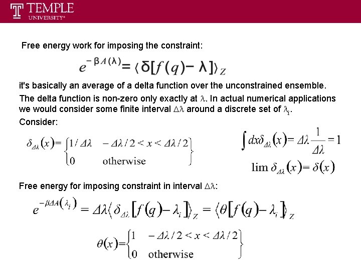
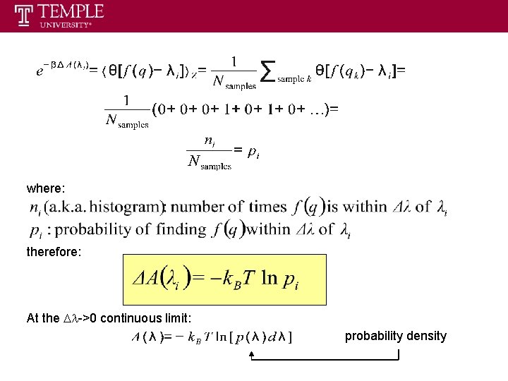
Free energy work for imposing the constraint: it's basically an average of a delta function over the unconstrained ensemble. The delta function is non-zero only exactly at l. In actual numerical applications we would consider some finite interval Dl around a discrete set of li. Consider: Free energy for imposing constraint in interval Dl:

where: therefore: At the Dl->0 continuous limit: probability density

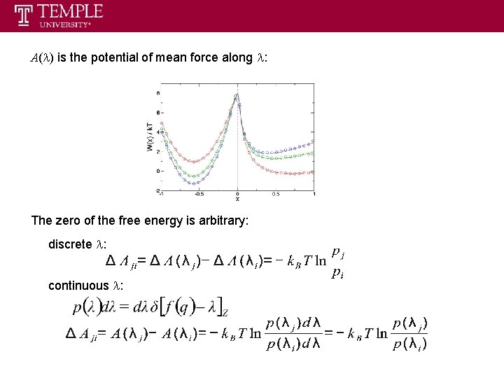
A(l) is the potential of mean force along l: The zero of the free energy is arbitrary: discrete l: continuous l:

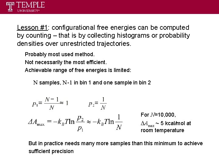
Lesson #1: configurational free energies can be computed by counting – that is by collecting histograms or probability densities over unrestricted trajectories. Probably most used method. Not necessarily the most efficient. Achievable range of free energies is limited: N samples, N-1 in bin 1 and one sample in bin 2 For N=10, 000, DAmax ~ 5 kcal/mol at room temperature But in practice needs many more samples than this minimum to achieve sufficient precision

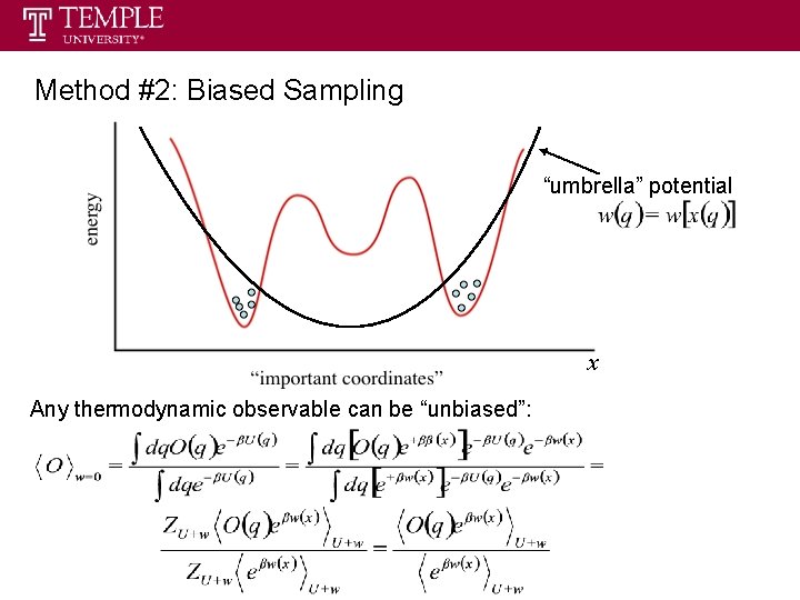
Method #2: Biased Sampling “umbrella” potential x Any thermodynamic observable can be “unbiased”:

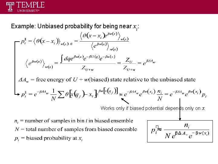
Example: Unbiased probability for being near xi: Works only if biased potential depends only on x

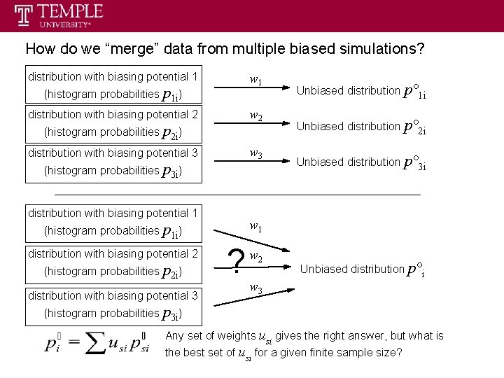
How do we “merge” data from multiple biased simulations? distribution with biasing potential 1 w 1 (histogram probabilities p 1 i) w 2 distribution with biasing potential 2 (histogram probabilities p 2 i) w 3 distribution with biasing potential 3 (histogram probabilities p 3 i) distribution with biasing potential 1 (histogram probabilities p 2 i) distribution with biasing potential 3 Unbiased distribution p° 2 i Unbiased distribution p° 3 i w 1 (histogram probabilities p 1 i) distribution with biasing potential 2 Unbiased distribution p° 1 i ? w 2 Unbiased distribution p°i w 3 (histogram probabilities p 3 i) Any set of weights usi gives the right answer, but what is the best set of usi for a given finite sample size?

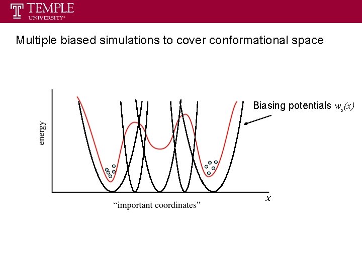
Multiple biased simulations to cover conformational space Biasing potentials ws(x) x

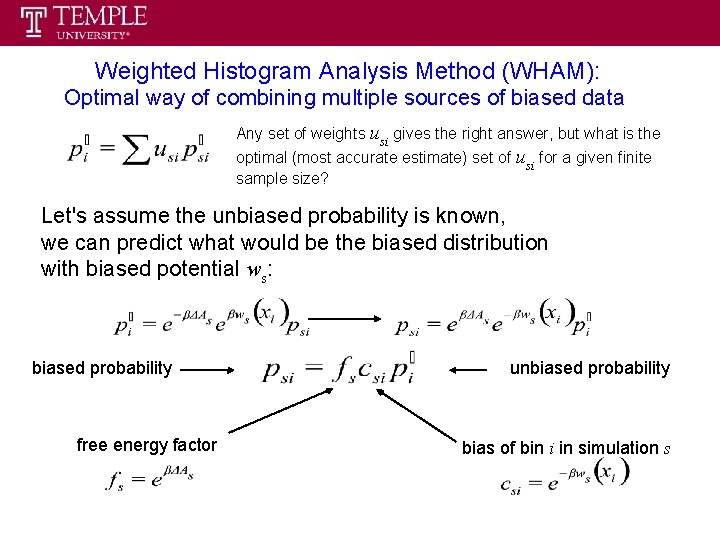
Weighted Histogram Analysis Method (WHAM): Optimal way of combining multiple sources of biased data Any set of weights usi gives the right answer, but what is the optimal (most accurate estimate) set of usi for a given finite sample size? Let's assume the unbiased probability is known, we can predict what would be the biased distribution with biased potential ws: biased probability free energy factor unbiased probability bias of bin i in simulation s

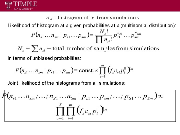
Likelihood of histogram at s given probabilities at s (multinomial distribution): In terms of unbiased probabilties: Joint likelihood of the histograms from all simulations:

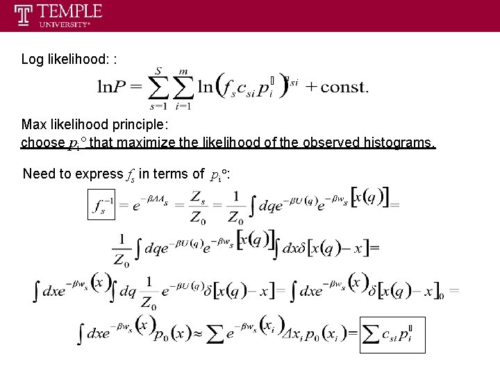
Log likelihood: : Max likelihood principle: choose pi° that maximize the likelihood of the observed histograms. Need to express fs in terms of pi°:

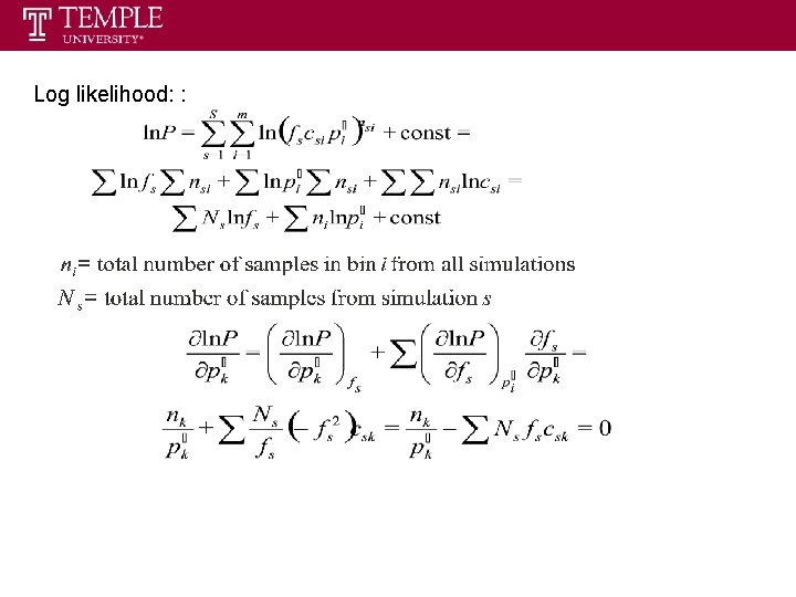
Log likelihood: :

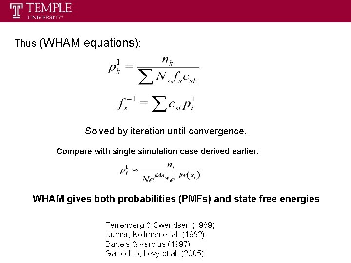
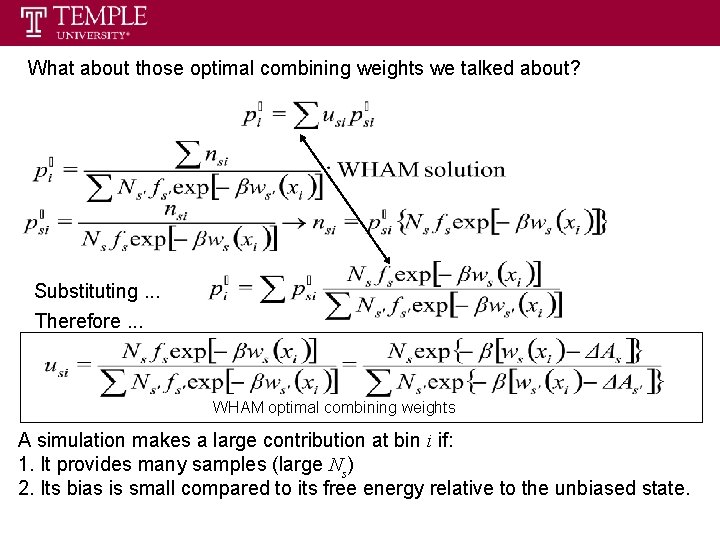
Thus (WHAM equations): Solved by iteration until convergence. Compare with single simulation case derived earlier: WHAM gives both probabilities (PMFs) and state free energies Ferrenberg & Swendsen (1989) Kumar, Kollman et al. (1992) Bartels & Karplus (1997) Gallicchio, Levy et al. (2005)

What about those optimal combining weights we talked about? Substituting. . . Therefore. . . WHAM optimal combining weights A simulation makes a large contribution at bin i if: 1. It provides many samples (large Ns) 2. Its bias is small compared to its free energy relative to the unbiased state.

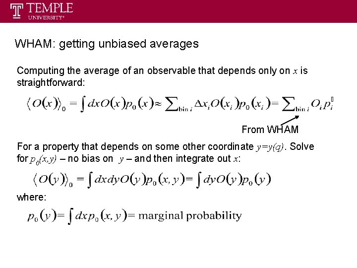
WHAM: getting unbiased averages Computing the average of an observable that depends only on x is straightforward: From WHAM For a property that depends on some other coordinate y=y(q). Solve for p 0(x, y) – no bias on y – and then integrate out x: where:

Some WHAM Applications for PMFs PMF of Alanine Dipeptide Chekmarev, Ishida, & Levy (2004) J. Phys. Chem. B 108: 19487 -19495

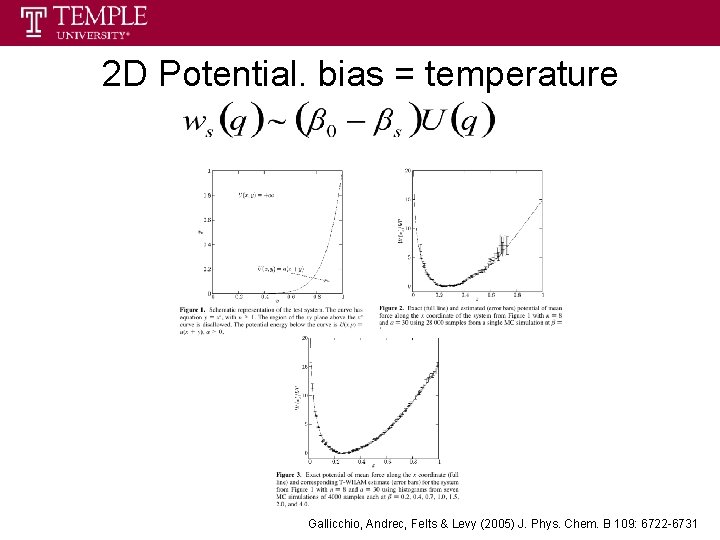
2 D Potential. bias = temperature Gallicchio, Andrec, Felts & Levy (2005) J. Phys. Chem. B 109: 6722 -6731

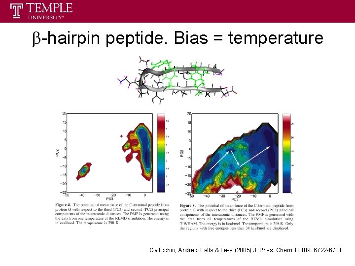
b-hairpin peptide. Bias = temperature Gallicchio, Andrec, Felts & Levy (2005) J. Phys. Chem. B 109: 6722 -6731

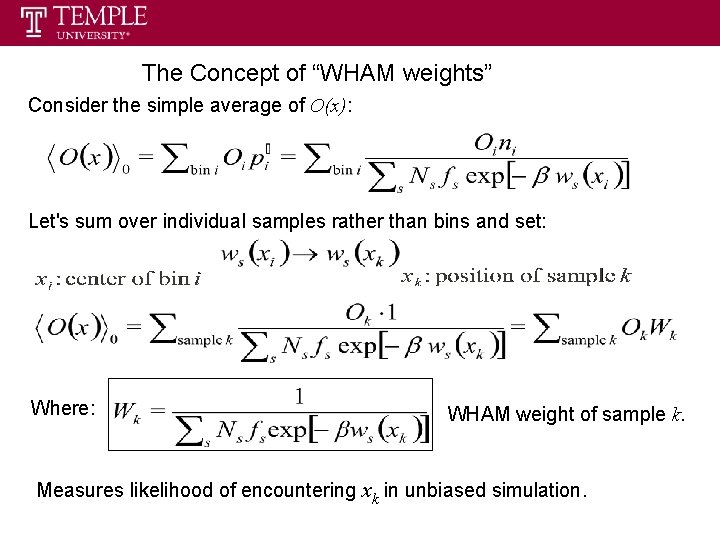
The Concept of “WHAM weights” Consider the simple average of O(x): Let's sum over individual samples rather than bins and set: Where: WHAM weight of sample k. Measures likelihood of encountering xk in unbiased simulation.

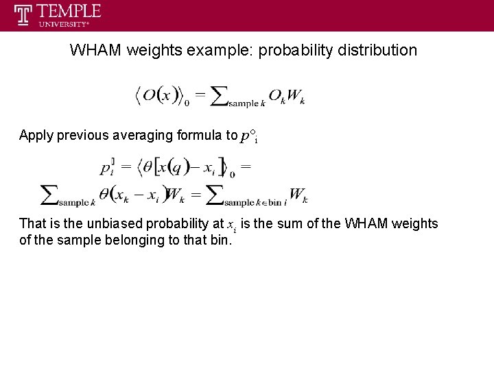
WHAM weights example: probability distribution Apply previous averaging formula to p°i That is the unbiased probability at xi is the sum of the WHAM weights of the sample belonging to that bin.

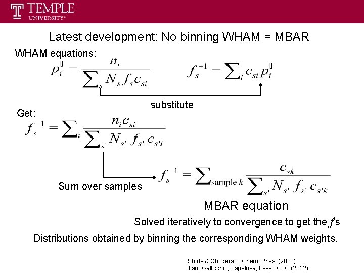
Latest development: No binning WHAM = MBAR WHAM equations: substitute Get: Sum over samples MBAR equation Solved iteratively to convergence to get the f's Distributions obtained by binning the corresponding WHAM weights. Shirts & Chodera J. Chem. Phys. (2008). Tan, Gallicchio, Lapelosa, Levy JCTC (2012).