Statistical Methods in HEP in particular Nuisance parameters

Statistical Methods in HEP, in particular. . . Nuisance parameters and systematic uncertainties Glen Cowan Royal Holloway, University of London g. cowan@rhul. ac. uk www. pp. rhul. ac. uk/~cowan RHUL HEP Seminar 22 March, 2006 A rehash my talk at the Io. P Half Day Meeting on Statistics in HEP University of Manchester, 16 November, 2005 Itself a rehash of PHYSTAT 2005, Oxford, September 2005 Glen Cowan RHUL HEP seminar, 22 March, 2006

Vague outline I. Nuisance parameters and systematic uncertainty II. Parameter measurement Frequentist Bayesian III. Estimating intervals (setting limits) Frequentist Bayesian IV. Comment on the D 0 result on Bs mixing V. Conclusions Glen Cowan RHUL HEP seminar, 22 March, 2006

Statistical vs. systematic errors Statistical errors: How much would the result fluctuate upon repetition of the measurement? Implies some set of assumptions to define probability of outcome of the measurement. Systematic errors: What is the uncertainty in my result due to uncertainty in my assumptions, e. g. , model (theoretical) uncertainty; modelling of measurement apparatus. The sources of error do not vary upon repetition of the measurement. Often result from uncertain value of, e. g. , calibration constants, efficiencies, etc. Glen Cowan RHUL HEP seminar, 22 March, 2006

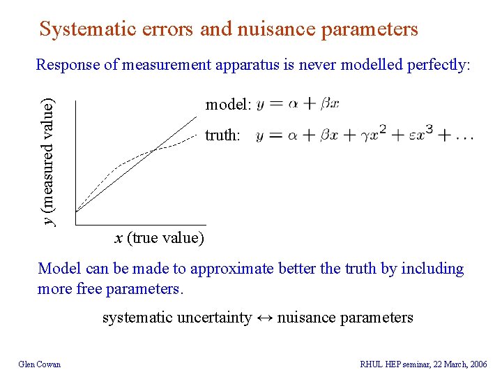
Systematic errors and nuisance parameters Response of measurement apparatus is never modelled perfectly: y (measured value) model: truth: x (true value) Model can be made to approximate better the truth by including more free parameters. systematic uncertainty ↔ nuisance parameters Glen Cowan RHUL HEP seminar, 22 March, 2006

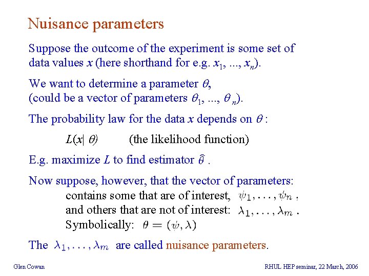
Nuisance parameters Suppose the outcome of the experiment is some set of data values x (here shorthand for e. g. x 1, . . . , xn). We want to determine a parameter , (could be a vector of parameters 1, . . . , n). The probability law for the data x depends on : L(x| ) (the likelihood function) E. g. maximize L to find estimator Now suppose, however, that the vector of parameters: contains some that are of interest, and others that are not of interest: Symbolically: The Glen Cowan are called nuisance parameters. RHUL HEP seminar, 22 March, 2006

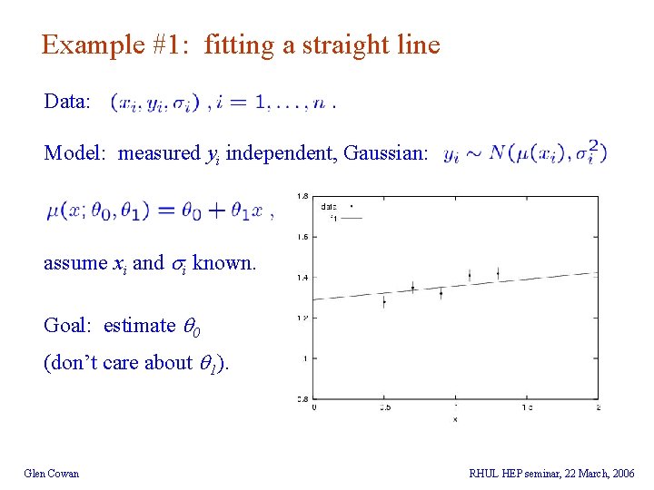
Example #1: fitting a straight line Data: Model: measured yi independent, Gaussian: assume xi and i known. Goal: estimate 0 (don’t care about 1). Glen Cowan RHUL HEP seminar, 22 March, 2006

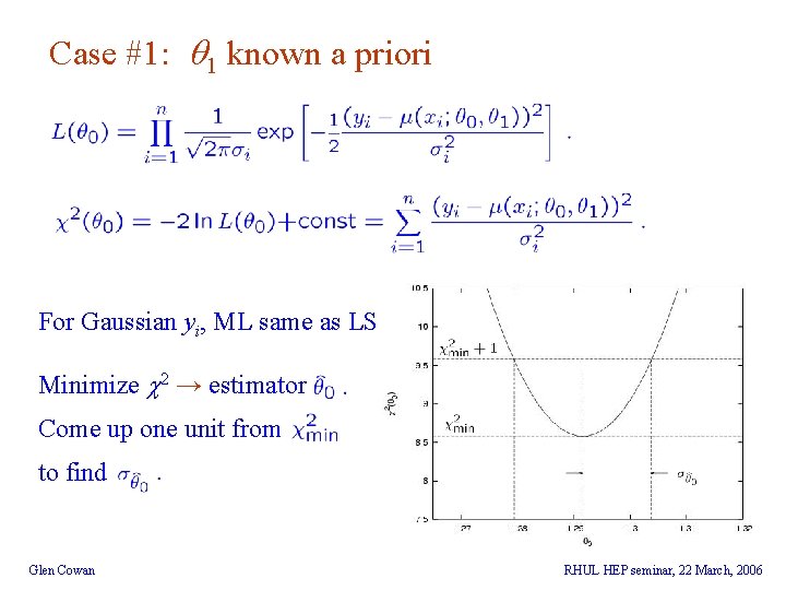
Case #1: 1 known a priori For Gaussian yi, ML same as LS Minimize c 2 → estimator Come up one unit from to find Glen Cowan RHUL HEP seminar, 22 March, 2006

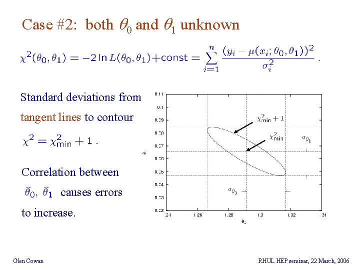
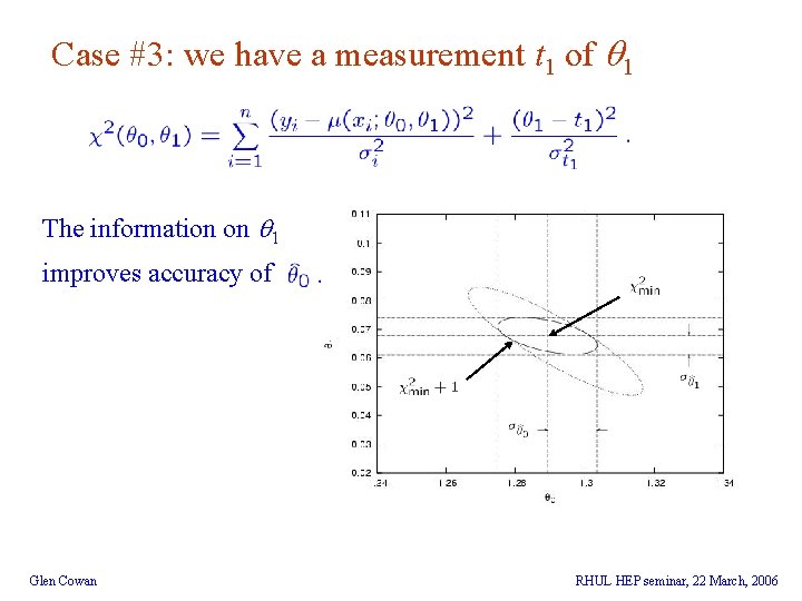
Case #2: both 0 and 1 unknown Standard deviations from tangent lines to contour Correlation between causes errors to increase. Glen Cowan RHUL HEP seminar, 22 March, 2006

Case #3: we have a measurement t 1 of 1 The information on 1 improves accuracy of Glen Cowan RHUL HEP seminar, 22 March, 2006

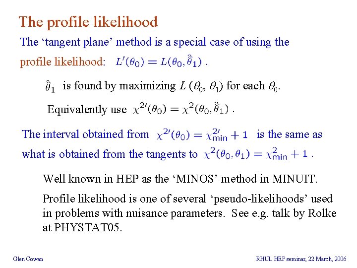
The profile likelihood The ‘tangent plane’ method is a special case of using the profile likelihood: is found by maximizing L ( 0, 1) for each 0. Equivalently use The interval obtained from is the same as what is obtained from the tangents to Well known in HEP as the ‘MINOS’ method in MINUIT. Profile likelihood is one of several ‘pseudo-likelihoods’ used in problems with nuisance parameters. See e. g. talk by Rolke at PHYSTAT 05. Glen Cowan RHUL HEP seminar, 22 March, 2006

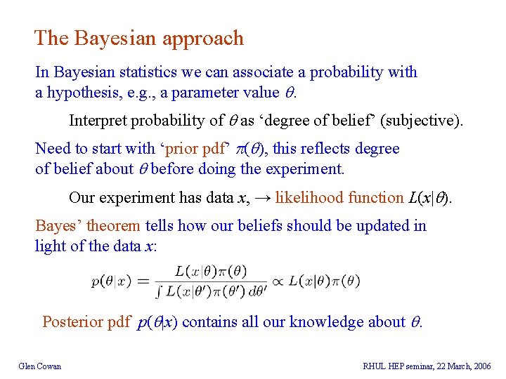
The Bayesian approach In Bayesian statistics we can associate a probability with a hypothesis, e. g. , a parameter value . Interpret probability of as ‘degree of belief’ (subjective). Need to start with ‘prior pdf’ ( ), this reflects degree of belief about before doing the experiment. Our experiment has data x, → likelihood function L(x| ). Bayes’ theorem tells how our beliefs should be updated in light of the data x: Posterior pdf p( |x) contains all our knowledge about . Glen Cowan RHUL HEP seminar, 22 March, 2006

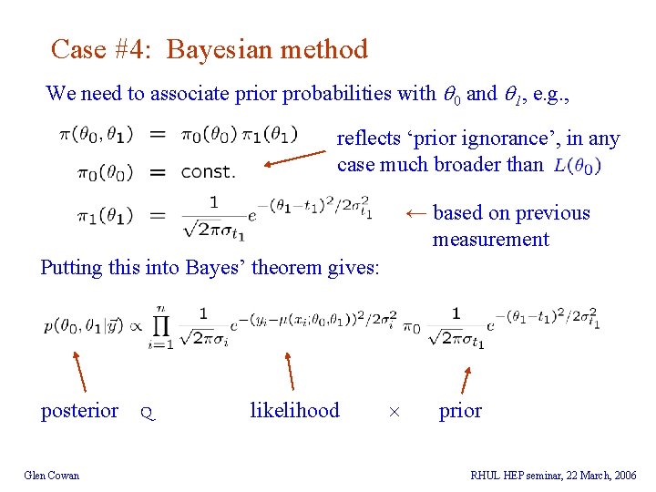
Case #4: Bayesian method We need to associate prior probabilities with 0 and 1, e. g. , reflects ‘prior ignorance’, in any case much broader than ← based on previous measurement Putting this into Bayes’ theorem gives: posterior Glen Cowan Q likelihood prior RHUL HEP seminar, 22 March, 2006

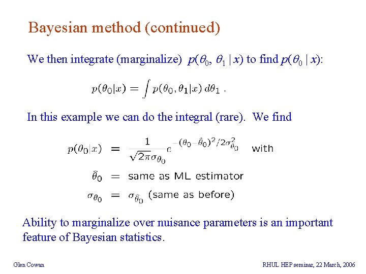
Bayesian method (continued) We then integrate (marginalize) p( 0, 1 | x) to find p( 0 | x): In this example we can do the integral (rare). We find Ability to marginalize over nuisance parameters is an important feature of Bayesian statistics. Glen Cowan RHUL HEP seminar, 22 March, 2006

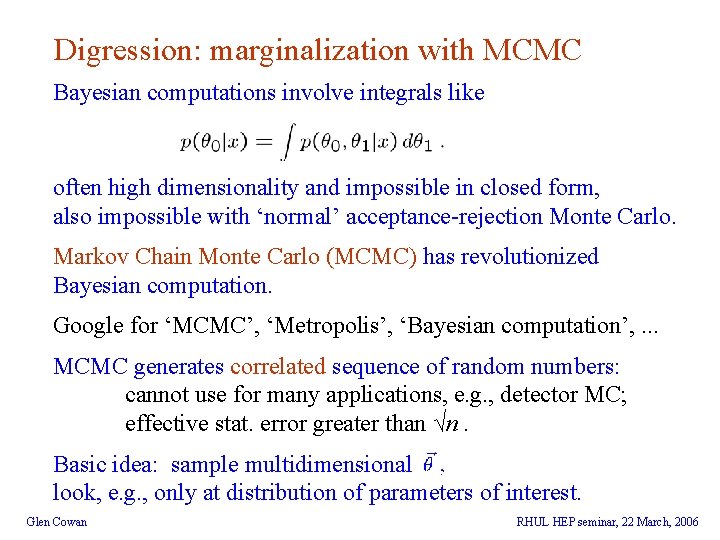
Digression: marginalization with MCMC Bayesian computations involve integrals like often high dimensionality and impossible in closed form, also impossible with ‘normal’ acceptance-rejection Monte Carlo. Markov Chain Monte Carlo (MCMC) has revolutionized Bayesian computation. Google for ‘MCMC’, ‘Metropolis’, ‘Bayesian computation’, . . . MCMC generates correlated sequence of random numbers: cannot use for many applications, e. g. , detector MC; effective stat. error greater than √n. Basic idea: sample multidimensional look, e. g. , only at distribution of parameters of interest. Glen Cowan RHUL HEP seminar, 22 March, 2006

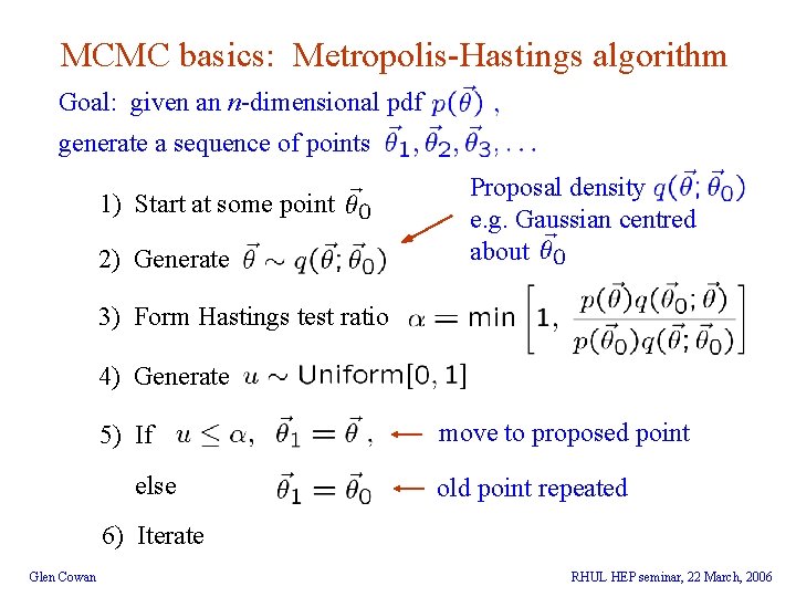
MCMC basics: Metropolis-Hastings algorithm Goal: given an n-dimensional pdf generate a sequence of points 1) Start at some point 2) Generate Proposal density e. g. Gaussian centred about 3) Form Hastings test ratio 4) Generate 5) If else move to proposed point old point repeated 6) Iterate Glen Cowan RHUL HEP seminar, 22 March, 2006

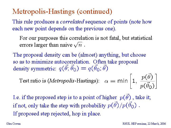
Metropolis-Hastings (continued) This rule produces a correlated sequence of points (note how each new point depends on the previous one). For our purposes this correlation is not fatal, but statistical errors larger than naive The proposal density can be (almost) anything, but choose so as to minimize autocorrelation. Often take proposal density symmetric: Test ratio is (Metropolis-Hastings): I. e. if the proposed step is to a point of higher if not, only take the step with probability If proposed step rejected, hop in place. Glen Cowan , take it; RHUL HEP seminar, 22 March, 2006

Metropolis-Hastings caveats Actually one can only prove that the sequence of points follows the desired pdf in the limit where it runs forever. There may be a “burn-in” period where the sequence does not initially follow Unfortunately there are few useful theorems to tell us when the sequence has converged. Look at trace plots, autocorrelation. Check result with different proposal density. If you think it’s converged, try it again with 10 times more points. Glen Cowan RHUL HEP seminar, 22 March, 2006

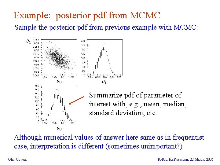
Example: posterior pdf from MCMC Sample the posterior pdf from previous example with MCMC: Summarize pdf of parameter of interest with, e. g. , mean, median, standard deviation, etc. Although numerical values of answer here same as in frequentist case, interpretation is different (sometimes unimportant? ) Glen Cowan RHUL HEP seminar, 22 March, 2006

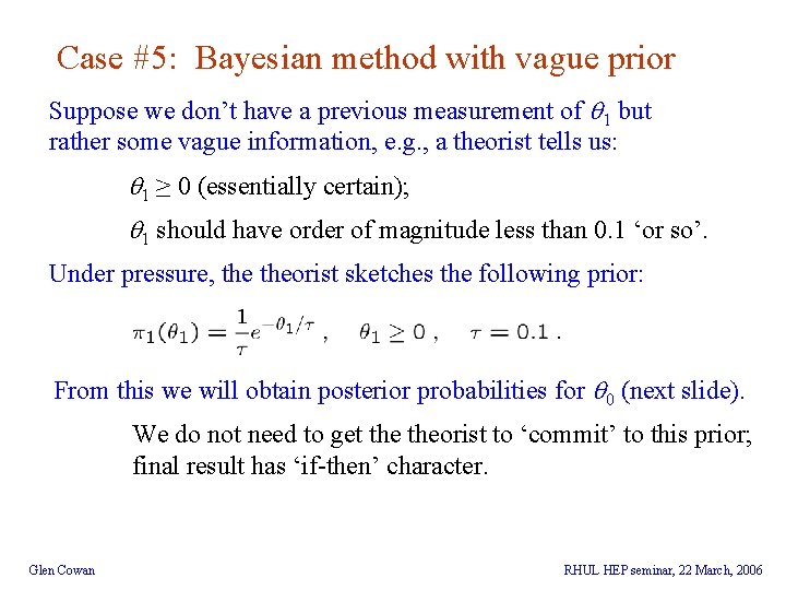
Case #5: Bayesian method with vague prior Suppose we don’t have a previous measurement of 1 but rather some vague information, e. g. , a theorist tells us: 1 ≥ 0 (essentially certain); 1 should have order of magnitude less than 0. 1 ‘or so’. Under pressure, theorist sketches the following prior: From this we will obtain posterior probabilities for 0 (next slide). We do not need to get theorist to ‘commit’ to this prior; final result has ‘if-then’ character. Glen Cowan RHUL HEP seminar, 22 March, 2006

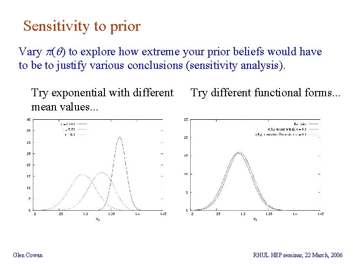
Sensitivity to prior Vary ( ) to explore how extreme your prior beliefs would have to be to justify various conclusions (sensitivity analysis). Try exponential with different mean values. . . Glen Cowan Try different functional forms. . . RHUL HEP seminar, 22 March, 2006

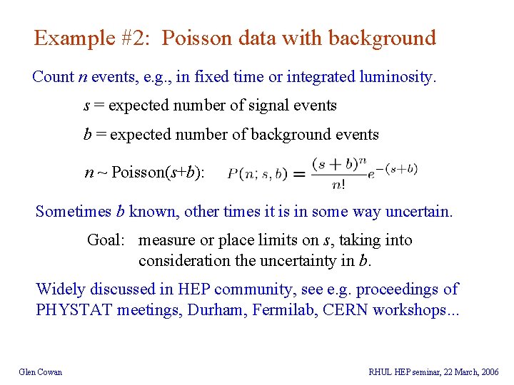
Example #2: Poisson data with background Count n events, e. g. , in fixed time or integrated luminosity. s = expected number of signal events b = expected number of background events n ~ Poisson(s+b): Sometimes b known, other times it is in some way uncertain. Goal: measure or place limits on s, taking into consideration the uncertainty in b. Widely discussed in HEP community, see e. g. proceedings of PHYSTAT meetings, Durham, Fermilab, CERN workshops. . . Glen Cowan RHUL HEP seminar, 22 March, 2006

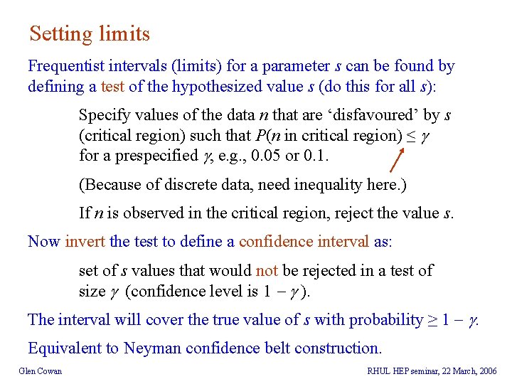
Setting limits Frequentist intervals (limits) for a parameter s can be found by defining a test of the hypothesized value s (do this for all s): Specify values of the data n that are ‘disfavoured’ by s (critical region) such that P(n in critical region) ≤ for a prespecified , e. g. , 0. 05 or 0. 1. (Because of discrete data, need inequality here. ) If n is observed in the critical region, reject the value s. Now invert the test to define a confidence interval as: set of s values that would not be rejected in a test of size (confidence level is 1 - ). The interval will cover the true value of s with probability ≥ 1 - . Equivalent to Neyman confidence belt construction. Glen Cowan RHUL HEP seminar, 22 March, 2006

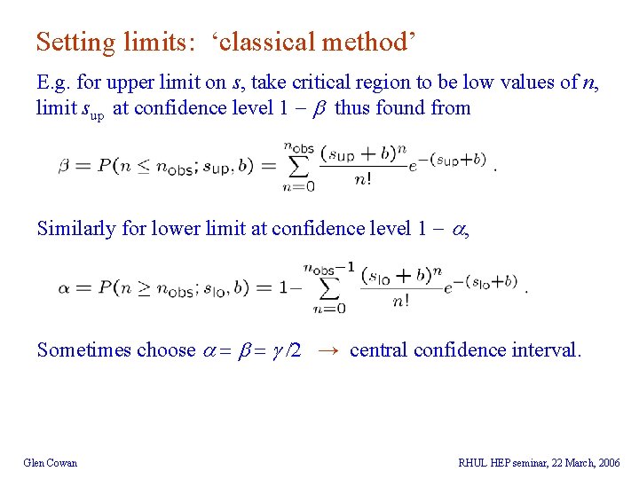
Setting limits: ‘classical method’ E. g. for upper limit on s, take critical region to be low values of n, limit sup at confidence level 1 - b thus found from Similarly for lower limit at confidence level 1 - a, Sometimes choose a = b = /2 → central confidence interval. Glen Cowan RHUL HEP seminar, 22 March, 2006

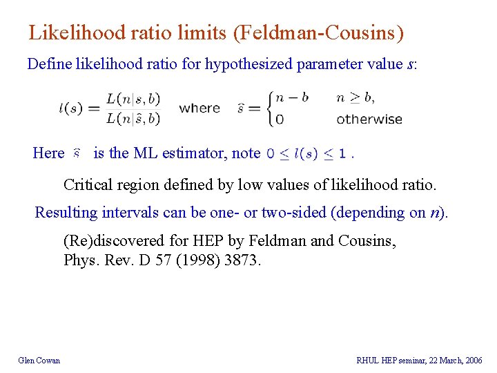
Likelihood ratio limits (Feldman-Cousins) Define likelihood ratio for hypothesized parameter value s: Here is the ML estimator, note Critical region defined by low values of likelihood ratio. Resulting intervals can be one- or two-sided (depending on n). (Re)discovered for HEP by Feldman and Cousins, Phys. Rev. D 57 (1998) 3873. Glen Cowan RHUL HEP seminar, 22 March, 2006

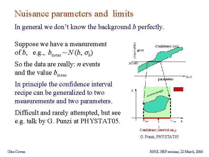
Nuisance parameters and limits In general we don’t know the background b perfectly. Suppose we have a measurement of b, e. g. , bmeas ~ N (b, b) So the data are really: n events and the value bmeas. In principle the confidence interval recipe can be generalized to two measurements and two parameters. Difficult and rarely attempted, but see e. g. talk by G. Punzi at PHYSTAT 05. G. Punzi, PHYSTAT 05 Glen Cowan RHUL HEP seminar, 22 March, 2006

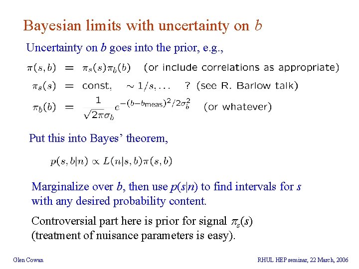
Bayesian limits with uncertainty on b Uncertainty on b goes into the prior, e. g. , Put this into Bayes’ theorem, Marginalize over b, then use p(s|n) to find intervals for s with any desired probability content. Controversial part here is prior for signal s(s) (treatment of nuisance parameters is easy). Glen Cowan RHUL HEP seminar, 22 March, 2006

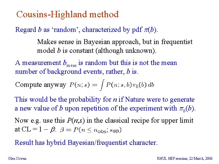
Cousins-Highland method Regard b as ‘random’, characterized by pdf (b). Makes sense in Bayesian approach, but in frequentist model b is constant (although unknown). A measurement bmeas is random but this is not the mean number of background events, rather, b is. Compute anyway This would be the probability for n if Nature were to generate a new value of b upon repetition of the experiment with b(b). Now e. g. use this P(n; s) in the classical recipe for upper limit at CL = 1 - b: Result has hybrid Bayesian/frequentist character. Glen Cowan RHUL HEP seminar, 22 March, 2006

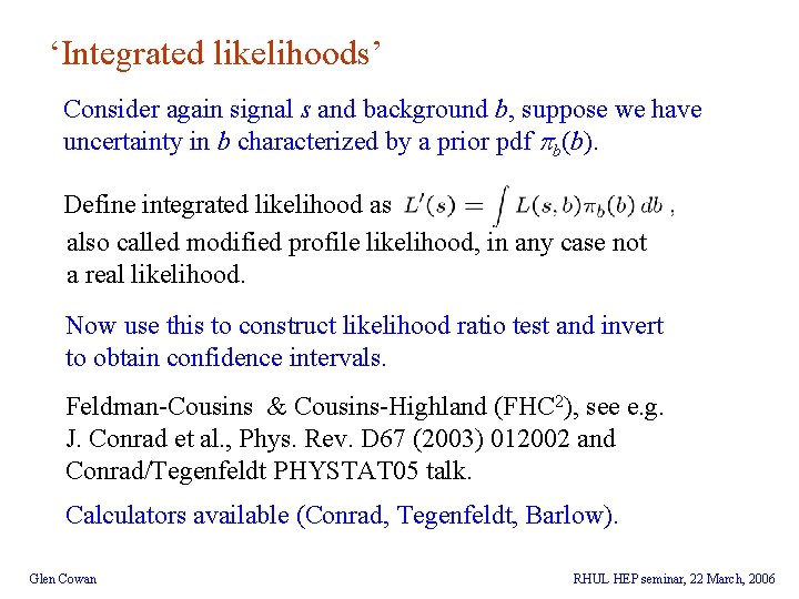
‘Integrated likelihoods’ Consider again signal s and background b, suppose we have uncertainty in b characterized by a prior pdf b(b). Define integrated likelihood as also called modified profile likelihood, in any case not a real likelihood. Now use this to construct likelihood ratio test and invert to obtain confidence intervals. Feldman-Cousins & Cousins-Highland (FHC 2), see e. g. J. Conrad et al. , Phys. Rev. D 67 (2003) 012002 and Conrad/Tegenfeldt PHYSTAT 05 talk. Calculators available (Conrad, Tegenfeldt, Barlow). Glen Cowan RHUL HEP seminar, 22 March, 2006

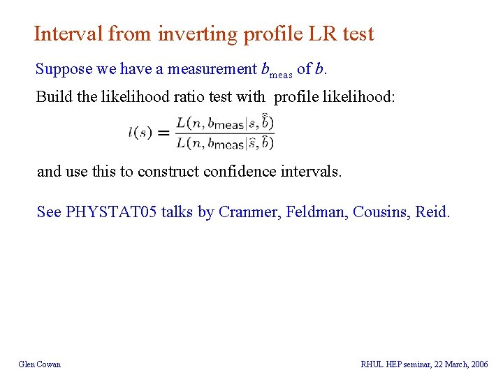
Interval from inverting profile LR test Suppose we have a measurement bmeas of b. Build the likelihood ratio test with profile likelihood: and use this to construct confidence intervals. See PHYSTAT 05 talks by Cranmer, Feldman, Cousins, Reid. Glen Cowan RHUL HEP seminar, 22 March, 2006

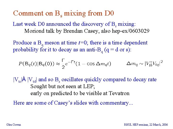
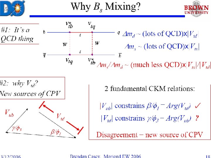
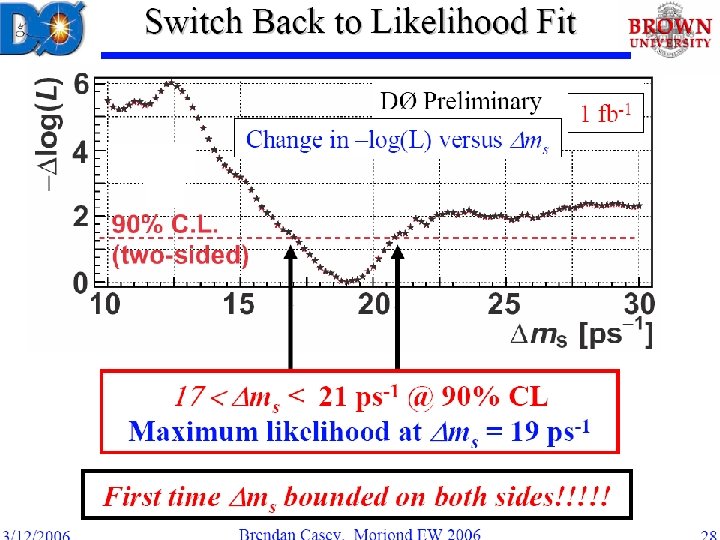
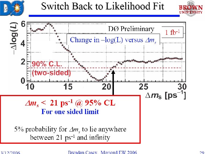
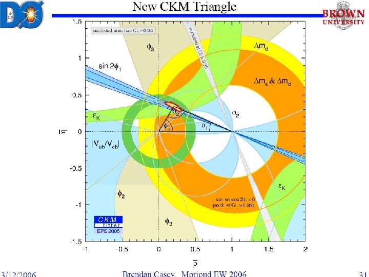
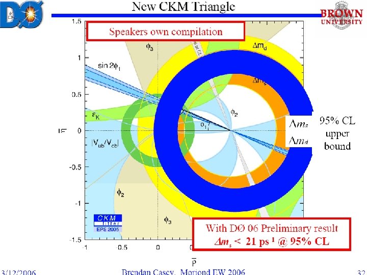
Comment on Bs mixing from D 0 Last week D 0 announced the discovery of Bs mixing: Moriond talk by Brendan Casey, also hep-ex/0603029 Produce a Bq meson at time t=0; there is a time dependent probability for it to decay as an anti-Bq (q = d or s): |Vts|À |Vtd| and so Bs oscillates quickly compared to decay rate Sought but not seen at LEP; early on predicted to be visible at Tevatron Here are some of Casey’s slides with commentary. . . Glen Cowan RHUL HEP seminar, 22 March, 2006

Glen Cowan Statistics in HEP, Io. P Half Day Meeting, 16 November 2005, Manchester

Glen Cowan Statistics in HEP, Io. P Half Day Meeting, 16 November 2005, Manchester

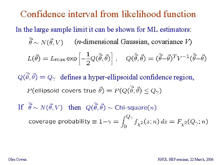
Confidence interval from likelihood function In the large sample limit it can be shown for ML estimators: (n-dimensional Gaussian, covariance V) defines a hyper-ellipsoidal confidence region, If Glen Cowan then RHUL HEP seminar, 22 March, 2006

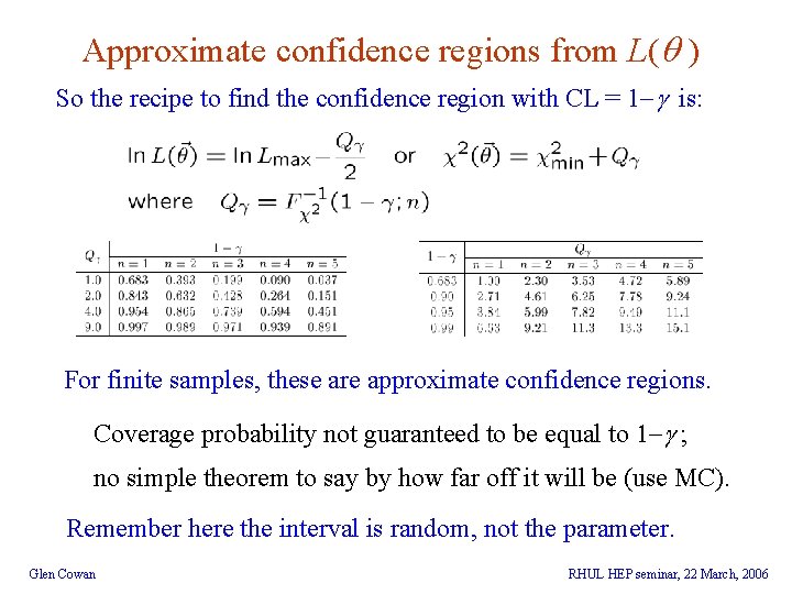
Approximate confidence regions from L( ) So the recipe to find the confidence region with CL = 1 - is: For finite samples, these are approximate confidence regions. Coverage probability not guaranteed to be equal to 1 - ; no simple theorem to say by how far off it will be (use MC). Remember here the interval is random, not the parameter. Glen Cowan RHUL HEP seminar, 22 March, 2006

Glen Cowan Statistics in HEP, Io. P Half Day Meeting, 16 November 2005, Manchester

Glen Cowan Statistics in HEP, Io. P Half Day Meeting, 16 November 2005, Manchester

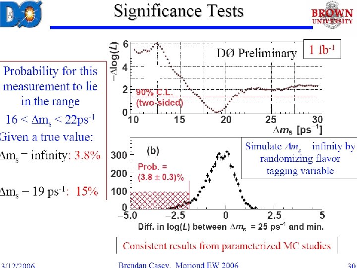
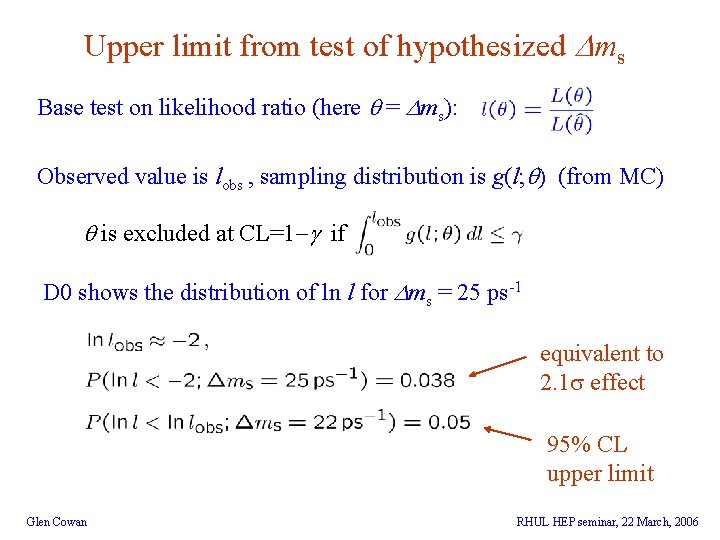
Upper limit from test of hypothesized ms Base test on likelihood ratio (here = ms): Observed value is lobs , sampling distribution is g(l; ) (from MC) is excluded at CL=1 - if D 0 shows the distribution of ln l for ms = 25 ps-1 equivalent to 2. 1 effect 95% CL upper limit Glen Cowan RHUL HEP seminar, 22 March, 2006

Glen Cowan Statistics in HEP, Io. P Half Day Meeting, 16 November 2005, Manchester

Glen Cowan Statistics in HEP, Io. P Half Day Meeting, 16 November 2005, Manchester

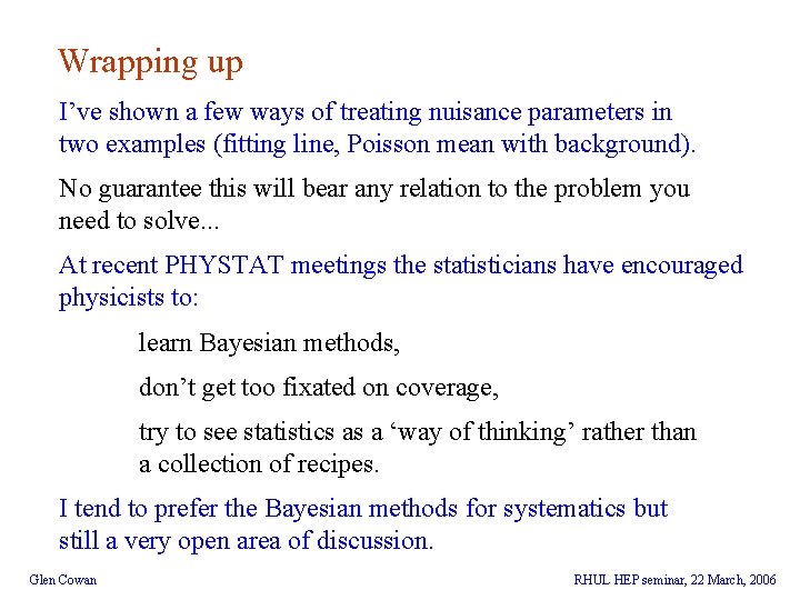
Wrapping up I’ve shown a few ways of treating nuisance parameters in two examples (fitting line, Poisson mean with background). No guarantee this will bear any relation to the problem you need to solve. . . At recent PHYSTAT meetings the statisticians have encouraged physicists to: learn Bayesian methods, don’t get too fixated on coverage, try to see statistics as a ‘way of thinking’ rather than a collection of recipes. I tend to prefer the Bayesian methods for systematics but still a very open area of discussion. Glen Cowan RHUL HEP seminar, 22 March, 2006