Fullyfrequentist handling of nuisance parameters in confidence limits

Fully-frequentist handling of nuisance parameters in confidence limits more details in: http: //www. samsi. info/200506/astro/workinggroup/phy/ and: http: //www. physics. ox. ac. uk/phystat 05/proceedings/files/Punzi_PHYSTAT 05_final. pdf Giovanni Punzi University and INFN-Pisa giovanni. punzi@pi. infn. it

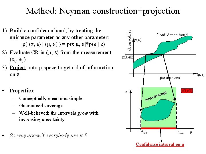
1) Build a confidence band, by treating the nuisance parameter as any other parameter: p( (x, e) | (µ, ) ) = p(x|µ, )*p(e | ) 2) Evaluate CR in (µ, ) from the measurement (x 0, e 0) 3) Project onto µ space to get rid of information on • Properties: – Conceptually clean and simple. – Guaranteed coverage. – Well-behaved: the intervals grow with increasing uncertainty • So why doesn’t everybody use it ? observables Method: Neyman construction+projection Confidence band (x, e) (x 0, e 0) (m, ) parameters (x 0, e 0) ge vera rco ove m min m max Confidence interval on µ m

Issues with the Neyman+projection • Overcoverage – Can be huge if you are not careful • Behavior when 0 – The limit may not be what you like it to be. This is an issue of other methods, too. • Shape of intervals – Hard to control the shape of the projections. e. g. not obvious how to obtain upper limits. • CPU requirements – Need “clever” algorithms • Multidimensional complexity

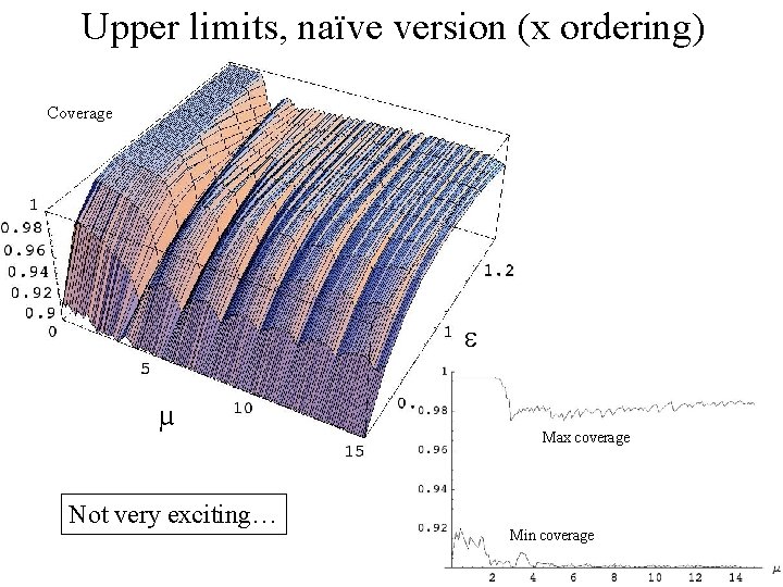
Upper limits, naïve version (x ordering) Coverage µ Not very exciting… Max coverage Min coverage

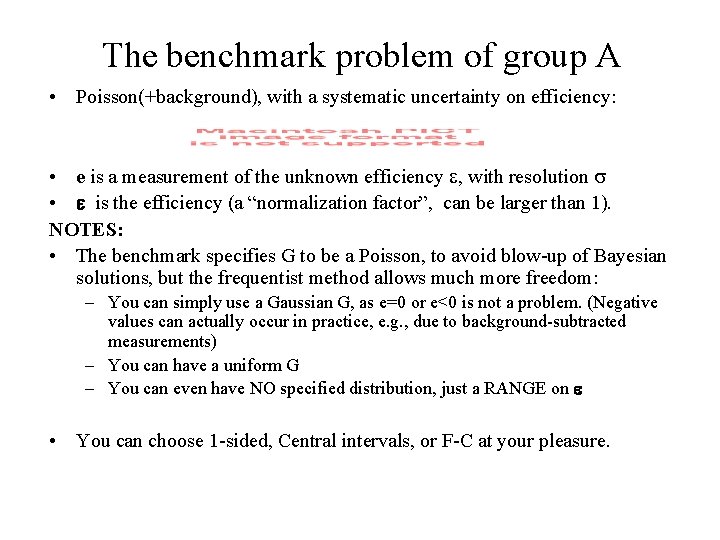
Past experience with projection method - No overwhelming enthusiasm in HEP. Most often replaced by some frequentist approximation: – Profile Likelihood – Smearing/averaging on the nuisance parameter (Cousins-Highland) • There were a few success stories: - Improved solution of the classical Poisson ratio problem: coordinated projections. [R. Cousins, Nucl. Instrum. Meth. A 417} 391 (1998)] - Final analysis of CHOOZ experiment: limits with systematics, prof-LR ordering [G. P. and G. Signorelli at PHYSTAT 02; Eur. Phys. J. C 27: 331(2003)] - Poisson+background with uncertainty: Hypothesis Test with prof-LR ordering [K. Cranmer at PHYSTAT 03, 05] - Poisson, uncertain efficiency: confidence region/any ordering/unspecified error distribution [G. P. at PHYSTAT 05]

My choice of Ordering Rule [Phystat 05] • I looked for an ordering rule in the space that would give me a desired ordering rule f 0(x) in the “interesting parameter” space. • I want the ordering to converge to the “local” ordering for each e, when 0 • The ordering is made not to depend on , as I am trying to ignore that information. This is handy because is saves computation (m 0) e Order as per e 2 Order as per e 1 A Þ Order in such a way as to integrate the same conditional probability at each e: This gives the ordering function: Where f 0(x) is the ordering function adopted for the 0 -systematics case N. B. I also do some clipping, mostly for computational reasons: when the tail probability for e becomes too small for given , I force it to low priority

The benchmark problem of group A • Poisson(+background), with a systematic uncertainty on efficiency: • e is a measurement of the unknown efficiency , with resolution • is the efficiency (a “normalization factor”, can be larger than 1). NOTES: • The benchmark specifies G to be a Poisson, to avoid blow-up of Bayesian solutions, but the frequentist method allows much more freedom: – You can simply use a Gaussian G, as e=0 or e<0 is not a problem. (Negative values can actually occur in practice, e. g. , due to background-subtracted measurements) – You can have a uniform G – You can even have NO specified distribution, just a RANGE on • You can choose 1 -sided, Central intervals, or F-C at your pleasure.

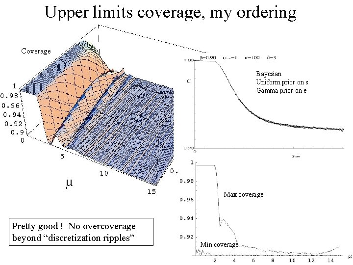
Upper limits coverage, my ordering Coverage coverage Bayesian Uniform prior on s Gamma prior on e Max coverage µ Max coverage Pretty good ! No overcoverage beyond “discretization ripples” Min coverage

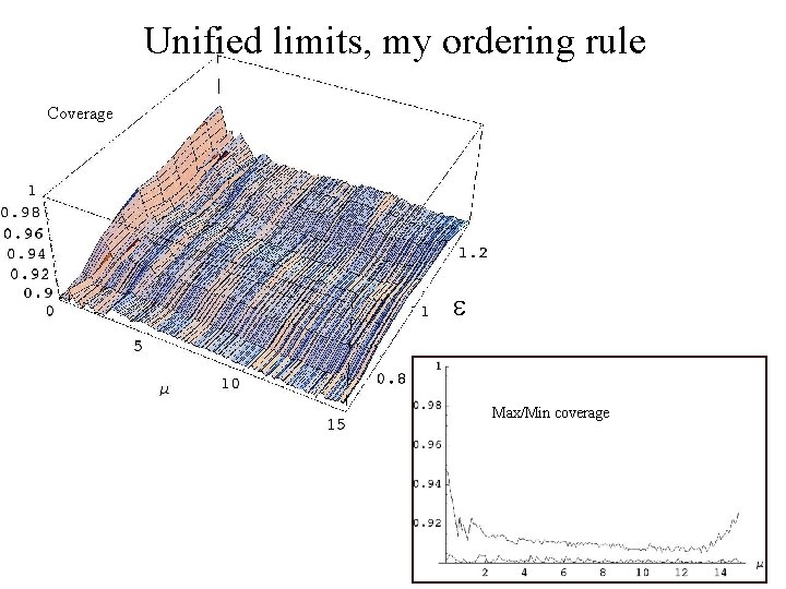
Unified limits, my ordering rule Coverage Max/Min coverage Average coverage

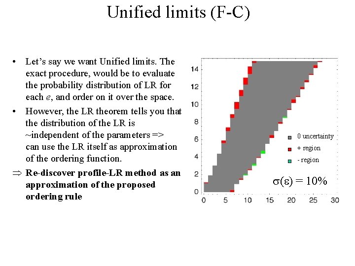
Unified limits (F-C) • Let’s say we want Unified limits. The exact procedure, would be to evaluate the probability distribution of LR for each e, and order on it over the space. • However, the LR theorem tells you that the distribution of the LR is ~independent of the parameters => can use the LR itself as approximation of the ordering function. Þ Re-discover profile-LR method as an approximation of the proposed ordering rule 0 uncertainty + region - region ( ) = 10%

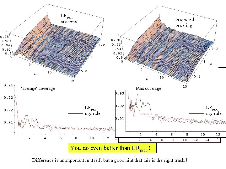
Coverage LRprof ordering proposed ordering µ ‘average’ coverage Max/Min coverage LRprof my rule Average coverage Yes ! You can do even better than LRprof ! You do even better than LRprof ! Difference is unimportant in itself, but a good hint that this is the right track ! LRprof my rule

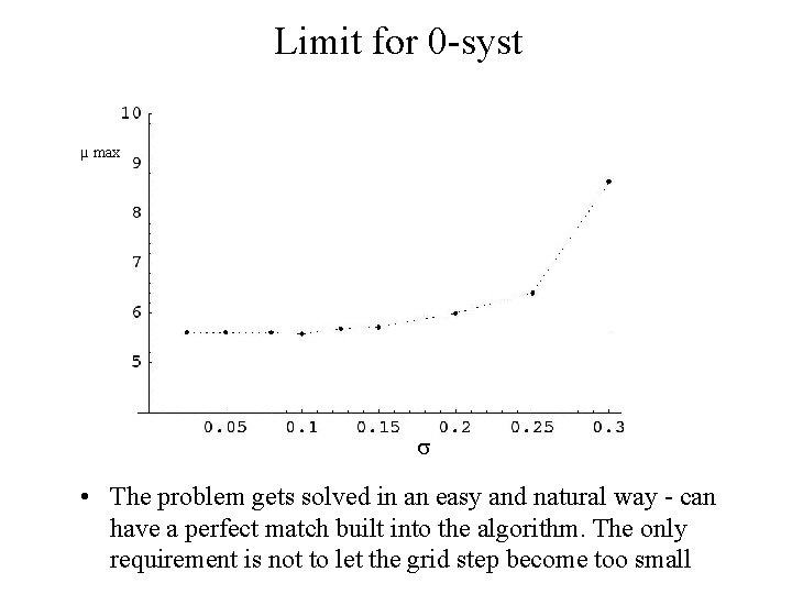
Limit for 0 -syst µ max • The problem gets solved in an easy and natural way - can have a perfect match built into the algorithm. The only requirement is not to let the grid step become too small

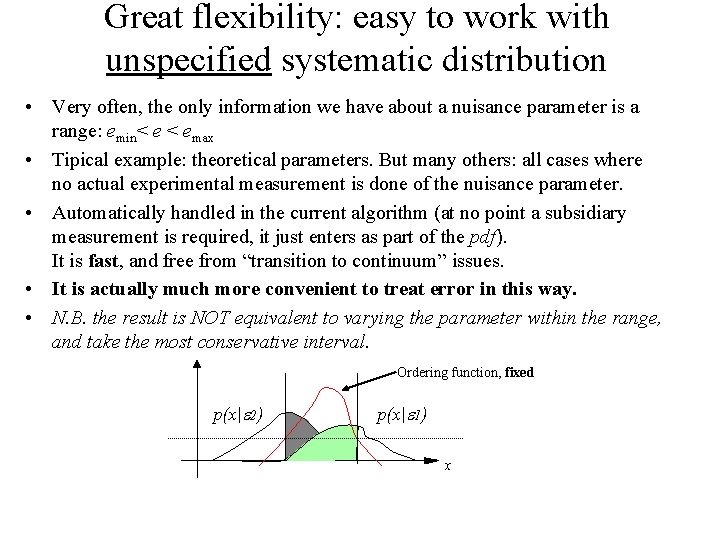
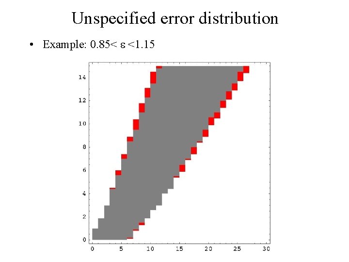
Great flexibility: easy to work with unspecified systematic distribution • Very often, the only information we have about a nuisance parameter is a range: emin< e < emax • Tipical example: theoretical parameters. But many others: all cases where no actual experimental measurement is done of the nuisance parameter. • Automatically handled in the current algorithm (at no point a subsidiary measurement is required, it just enters as part of the pdf). It is fast, and free from “transition to continuum” issues. • It is actually much more convenient to treat error in this way. • N. B. the result is NOT equivalent to varying the parameter within the range, and take the most conservative interval. Ordering function, fixed p(x| 2) p(x| 1) x

Unspecified error distribution • Example: 0. 85< <1. 15

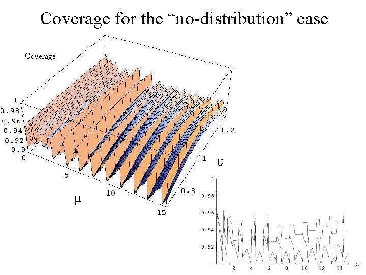
Coverage for the “no-distribution” case Coverage µ

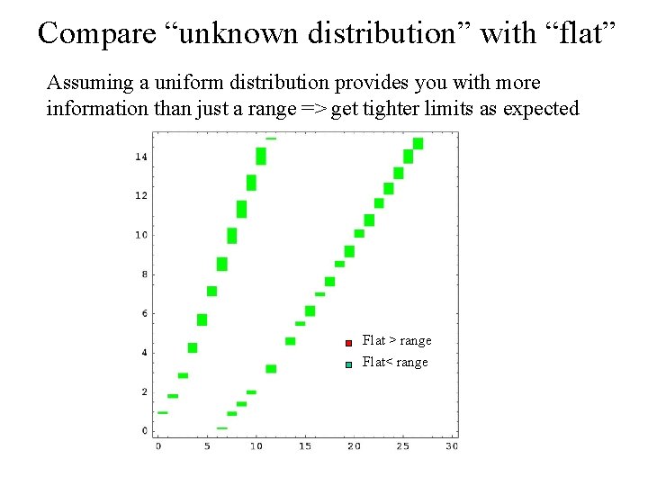
Compare “unknown distribution” with “flat” Assuming a uniform distribution provides you with more information than just a range => get tighter limits as expected Flat > range Flat< range

Computational Aspects 1) The ordering algorithm being independent of the nuisance parameters makes it much more convenient to perform the calculations • one can order just one time for each value of mu, and then go through the same list every time, just skipping the elements that are clipped off for that particular value of the nuisance parameter. 2) The clipping reduces the amount of space to be searched 3) The chosen ordering naturally provides acceptance regions that are slowly varying with the subsidiary measurement=> need to sample only a very small number of points. (used 10, but 2 would be enough) 4) For the same reasons, when multiple nuisance parameters are present, large combinatorics is unnecessary: sampling the corners of the hyperrectangle is sufficient (plus maybe additional random points). 5) The discreteness limitation further reduces the time needed. 6) Uncertainty given as ranges are extremely fast to calculate - one might willingly use this method for fast evaluation. They are also immune to the 0 -limit problem, so need no adjustments.

Conclusion …waiting for THE MATRIX