Statistical Machine Translation Part IV LogLinear Models Alexander

Statistical Machine Translation Part IV – Log-Linear Models Alexander Fraser CIS, LMU München 2020 -05 -06 Machine Translation

Where we have been • Solving a problem where we are predicting a structured output: – Problem definition – Evaluation, i. e. , how will we evaluate progress? – Model – Training = parameter estimation • Still to come: – Search (= decoding, for SMT)

Where we are going today • The generative models we have seen so far are good, but we can do better – Switch to discriminative models (this will be defined later) – We will see that this frees us from the structure of the generative model! • We can concentrate on new knowledge sources • Also, no more annoying open parameters – Discriminative models are used practically everywhere in NLP these days (including in deep learning approaches)

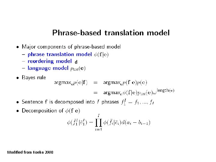
Outline • • • Recap: original phrase-based model Optimizing parameters Deriving the log-linear model Tuning the log-linear model Adding new features

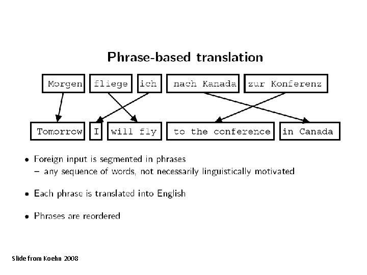
Slide from Koehn 2008

d Modified from Koehn 2008

Outline • • • Recap Optimizing parameters Deriving the log-linear model Tuning the log-linear model Adding new features

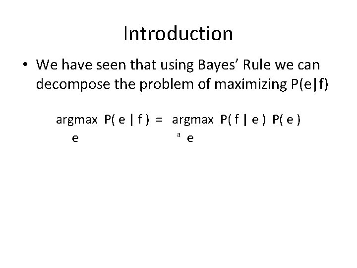
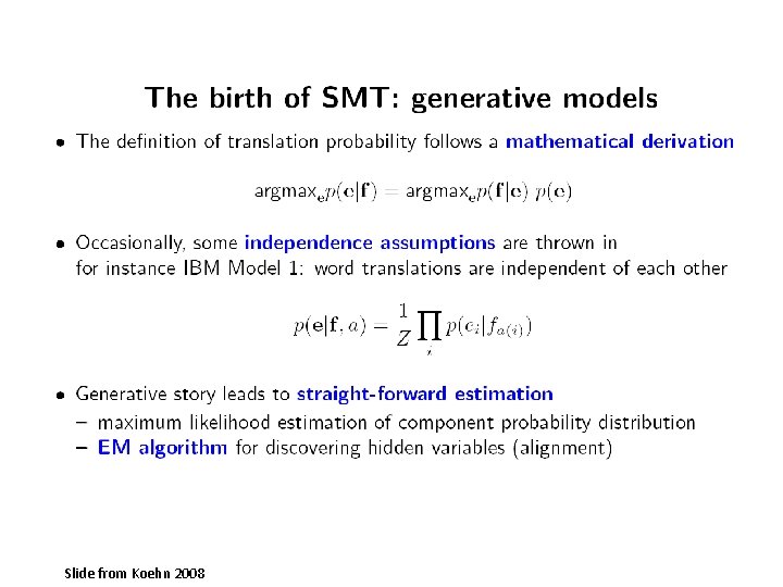
Introduction • We have seen that using Bayes’ Rule we can decompose the problem of maximizing P(e|f) argmax P( e | f ) = argmax P( f | e ) P( e ) e e

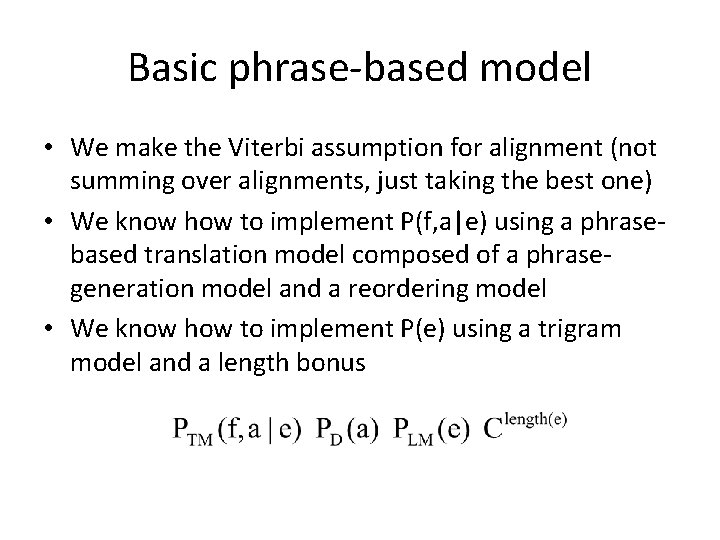
Basic phrase-based model • We make the Viterbi assumption for alignment (not summing over alignments, just taking the best one) • We know how to implement P(f, a|e) using a phrasebased translation model composed of a phrasegeneration model and a reordering model • We know how to implement P(e) using a trigram model and a length bonus

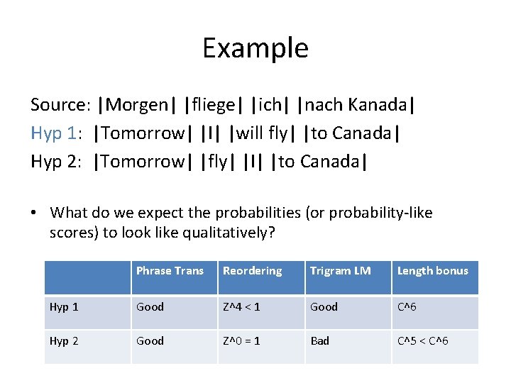
Example Source: |Morgen| |fliege| |ich| |nach Kanada| Hyp 1: |Tomorrow| |I| |will fly| |to Canada| Hyp 2: |Tomorrow| |fly| |I| |to Canada| • What do we expect the probabilities (or probability-like scores) to look like qualitatively? Phrase Trans Reordering Trigram LM Length bonus Hyp 1 Good Z^4 < 1 Good C^6 Hyp 2 Good Z^0 = 1 Bad C^5 < C^6

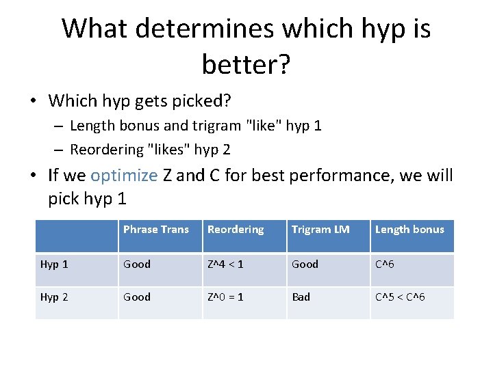
What determines which hyp is better? • Which hyp gets picked? – Length bonus and trigram "like" hyp 1 – Reordering "likes" hyp 2 • If we optimize Z and C for best performance, we will pick hyp 1 Phrase Trans Reordering Trigram LM Length bonus Hyp 1 Good Z^4 < 1 Good C^6 Hyp 2 Good Z^0 = 1 Bad C^5 < C^6

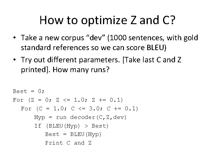
How to optimize Z and C? • Take a new corpus “dev” (1000 sentences, with gold standard references so we can score BLEU) • Try out different parameters. [Take last C and Z printed]. How many runs? Best = 0; For (Z = 0; Z <= 1. 0; Z += 0. 1) For (C = 1. 0; C <= 3. 0; C += 0. 1) Hyp = run decoder(C, Z, dev) If (BLEU(Hyp) > Best) Best = BLEU(Hyp) Print C and Z

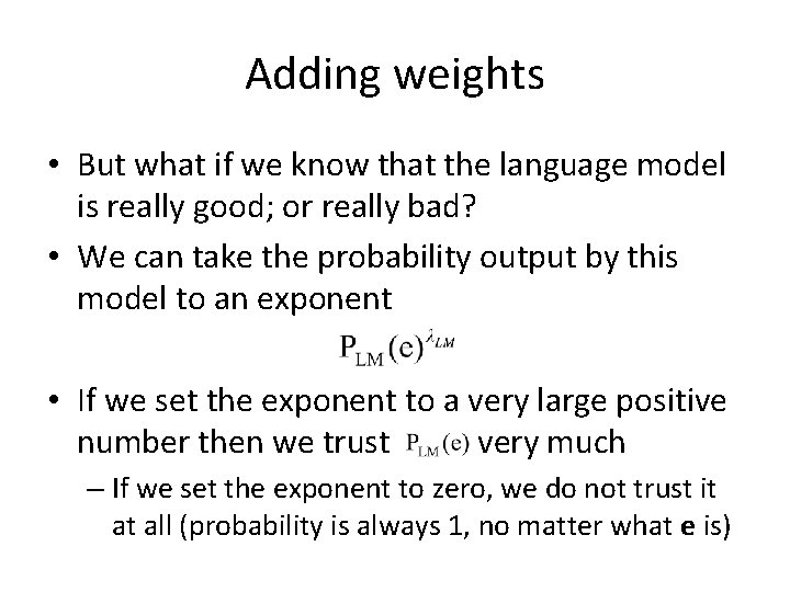
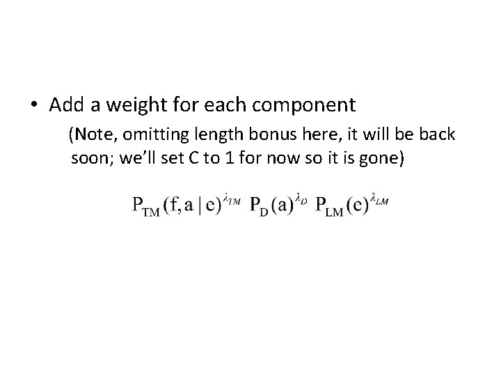
Adding weights • But what if we know that the language model is really good; or really bad? • We can take the probability output by this model to an exponent • If we set the exponent to a very large positive number then we trust very much – If we set the exponent to zero, we do not trust it at all (probability is always 1, no matter what e is)

• Add a weight for each component (Note, omitting length bonus here, it will be back soon; we’ll set C to 1 for now so it is gone)

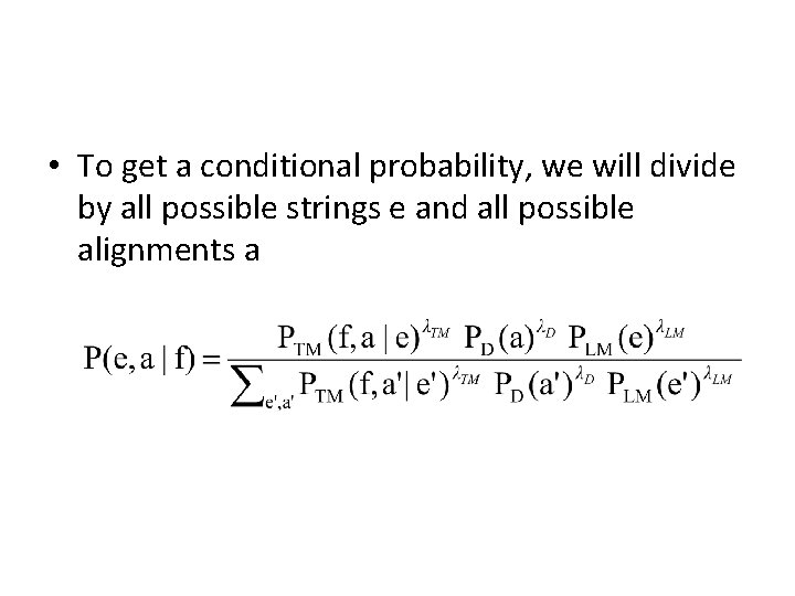
• To get a conditional probability, we will divide by all possible strings e and all possible alignments a

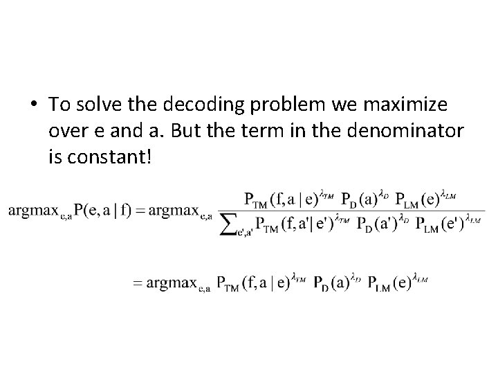
• To solve the decoding problem we maximize over e and a. But the term in the denominator is constant!

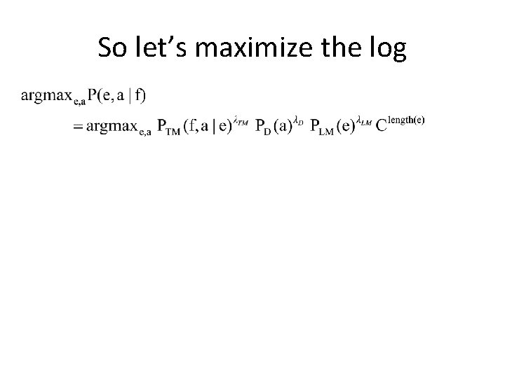
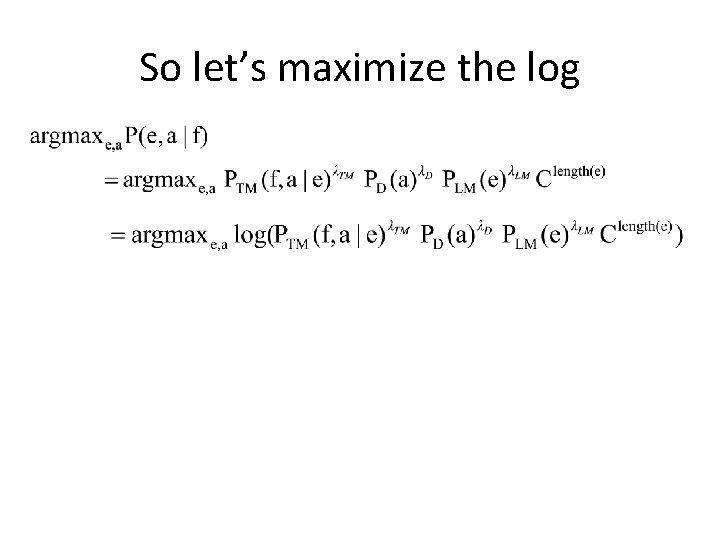
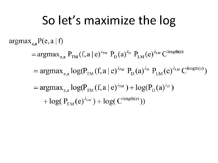
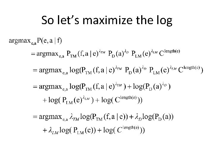
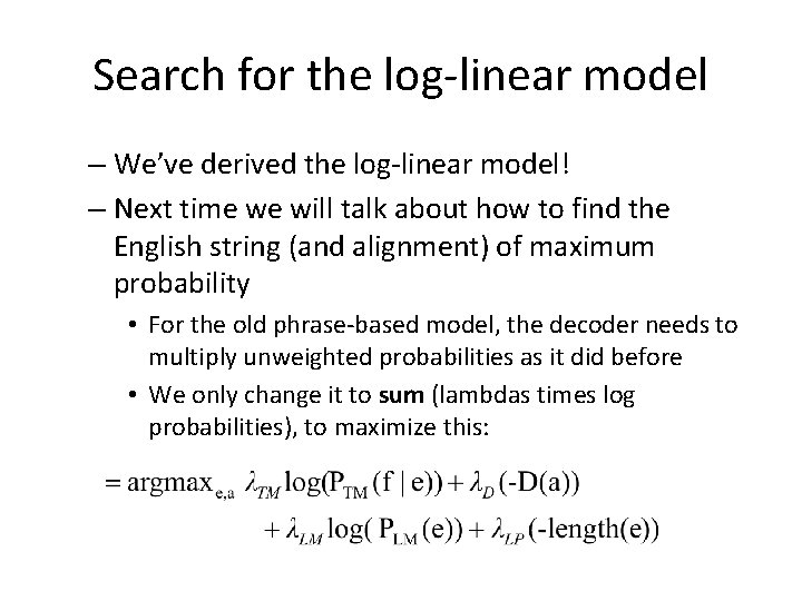
• Now let's add C back in and take the log (see formulation in a couple of slides) • We now have two problems – Optimize Z and C and the three lambdas – Exponentiation is slow • Let’s solve this one first…

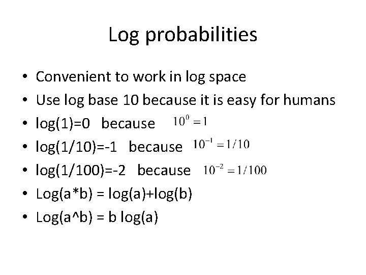
Log probabilities • • Convenient to work in log space Use log base 10 because it is easy for humans log(1)=0 because log(1/10)=-1 because log(1/100)=-2 because Log(a*b) = log(a)+log(b) Log(a^b) = b log(a)

So let’s maximize the log

So let’s maximize the log

So let’s maximize the log

So let’s maximize the log

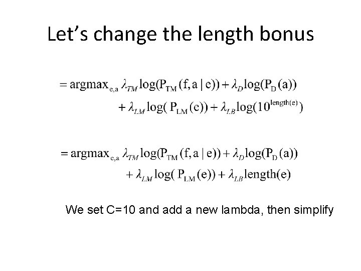
Let’s change the length bonus We set C=10 and add a new lambda, then simplify

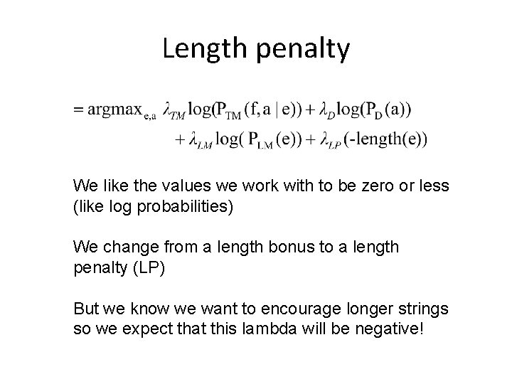
Length penalty We like the values we work with to be zero or less (like log probabilities) We change from a length bonus to a length penalty (LP) But we know we want to encourage longer strings so we expect that this lambda will be negative!

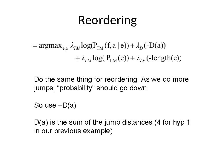
Reordering Do the same thing for reordering. As we do more jumps, “probability” should go down. So use –D(a) is the sum of the jump distances (4 for hyp 1 in our previous example)

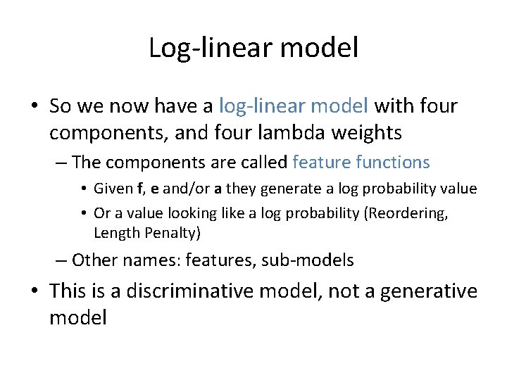
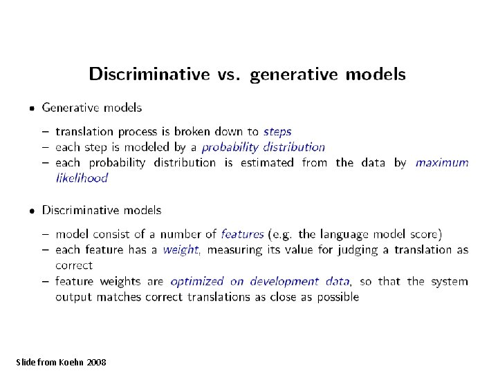
Log-linear model • So we now have a log-linear model with four components, and four lambda weights – The components are called feature functions • Given f, e and/or a they generate a log probability value • Or a value looking like a log probability (Reordering, Length Penalty) – Other names: features, sub-models • This is a discriminative model, not a generative model

Slide from Koehn 2008

Slide from Koehn 2008

Search for the log-linear model – We’ve derived the log-linear model! – Next time we will talk about how to find the English string (and alignment) of maximum probability • For the old phrase-based model, the decoder needs to multiply unweighted probabilities as it did before • We only change it to sum (lambdas times log probabilities), to maximize this:

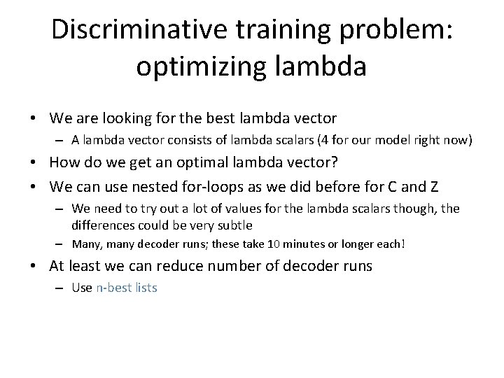
Discriminative training problem: optimizing lambda • We are looking for the best lambda vector – A lambda vector consists of lambda scalars (4 for our model right now) • How do we get an optimal lambda vector? • We can use nested for-loops as we did before for C and Z – We need to try out a lot of values for the lambda scalars though, the differences could be very subtle – Many, many decoder runs; these take 10 minutes or longer each! • At least we can reduce number of decoder runs – Use n-best lists

Slide from Koehn 2008

Slide from Koehn 2008

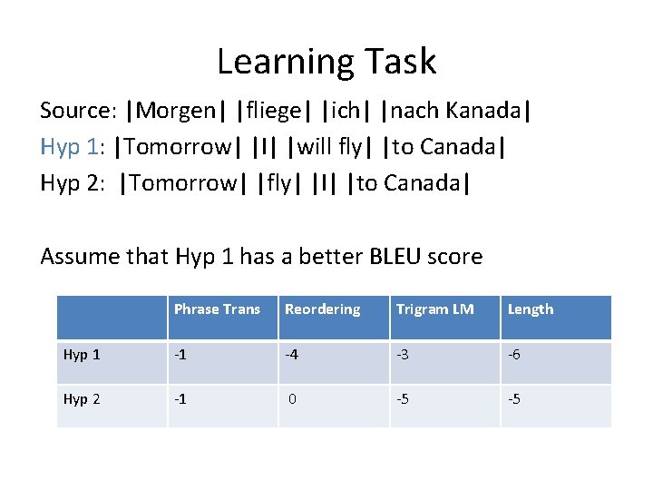
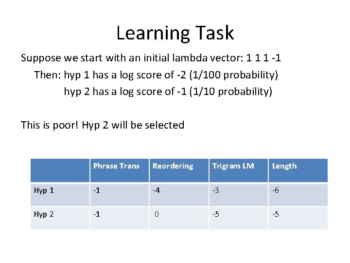
Learning Task Source: |Morgen| |fliege| |ich| |nach Kanada| Hyp 1: |Tomorrow| |I| |will fly| |to Canada| Hyp 2: |Tomorrow| |fly| |I| |to Canada| Assume that Hyp 1 has a better BLEU score Phrase Trans Reordering Trigram LM Length Hyp 1 -1 -4 -3 -6 Hyp 2 -1 0 -5 -5

Learning Task Suppose we start with an initial lambda vector: 1 1 1 -1 Then: hyp 1 has a log score of -2 (1/100 probability) hyp 2 has a log score of -1 (1/10 probability) This is poor! Hyp 2 will be selected Phrase Trans Reordering Trigram LM Length Hyp 1 -1 -4 -3 -6 Hyp 2 -1 0 -5 -5

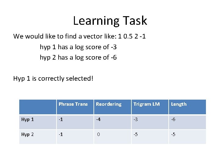
Learning Task We would like to find a vector like: 1 0. 5 2 -1 hyp 1 has a log score of -3 hyp 2 has a log score of -6 Hyp 1 is correctly selected! Phrase Trans Reordering Trigram LM Length Hyp 1 -1 -4 -3 -6 Hyp 2 -1 0 -5 -5

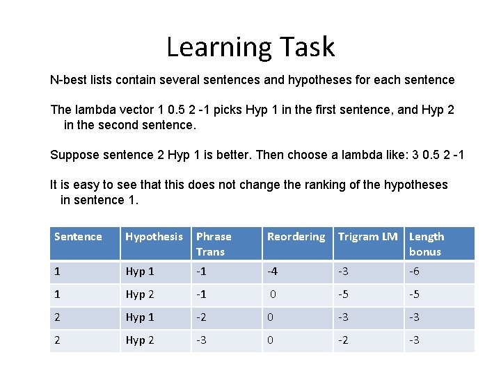
Learning Task N-best lists contain several sentences and hypotheses for each sentence The lambda vector 1 0. 5 2 -1 picks Hyp 1 in the first sentence, and Hyp 2 in the second sentence. Suppose sentence 2 Hyp 1 is better. Then choose a lambda like: 3 0. 5 2 -1 It is easy to see that this does not change the ranking of the hypotheses in sentence 1. Sentence Hypothesis Phrase Trans Reordering Trigram LM Length bonus 1 Hyp 1 -1 -4 -3 -6 1 Hyp 2 -1 0 -5 -5 2 Hyp 1 -2 0 -3 -3 2 Hyp 2 -3 0 -2 -3

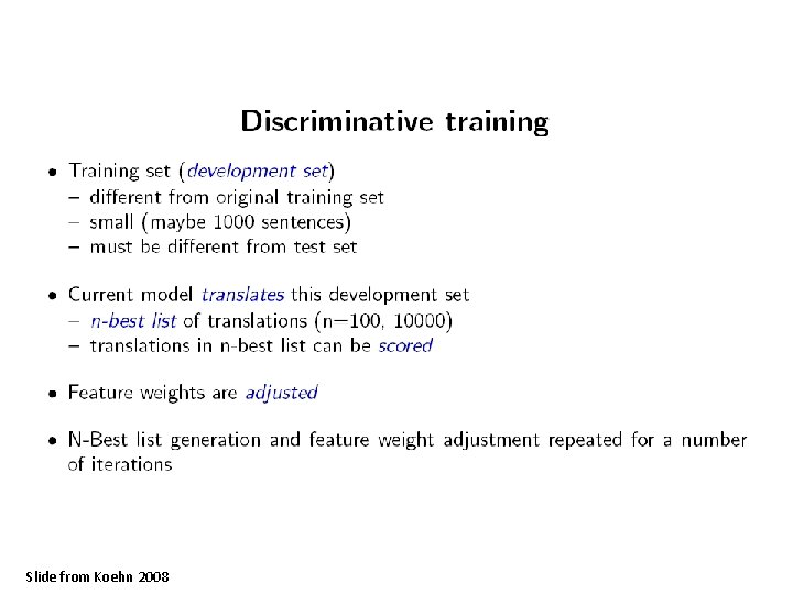
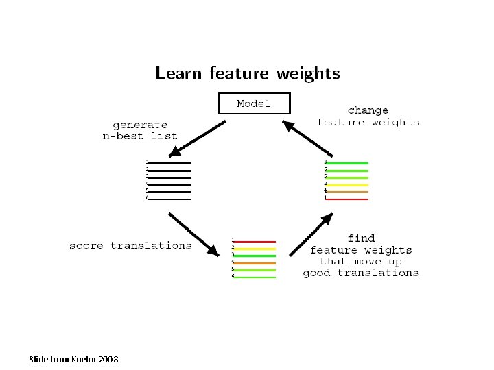
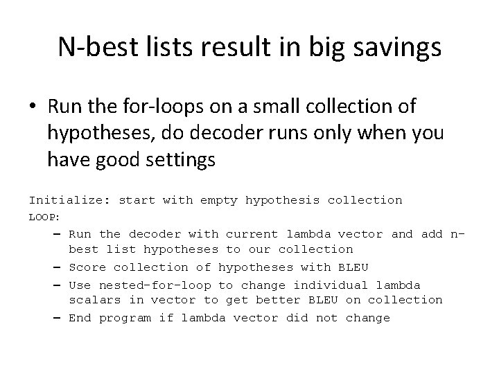
N-best lists result in big savings • Run the for-loops on a small collection of hypotheses, do decoder runs only when you have good settings Initialize: start with empty hypothesis collection LOOP: – Run the decoder with current lambda vector and add nbest list hypotheses to our collection – Score collection of hypotheses with BLEU – Use nested-for-loop to change individual lambda scalars in vector to get better BLEU on collection – End program if lambda vector did not change

• OK, so we know how to set the lambda vector for our feature functions – This means depending on the task we might, for instance, penalize reordering more or less – This is determined automatically by the performance on the dev corpus • But what about new features?

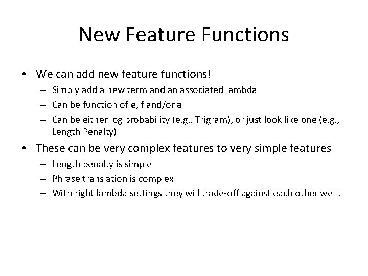
New Feature Functions • We can add new feature functions! – Simply add a new term and an associated lambda – Can be function of e, f and/or a – Can be either log probability (e. g. , Trigram), or just look like one (e. g. , Length Penalty) • These can be very complex features to very simple features – Length penalty is simple – Phrase translation is complex – With right lambda settings they will trade-off against each other well!

New Feature Functions • Features can overlap with one another! – In a generative model we do a sequence of steps, no overlapping allowed – In Model 1, you can’t pick a generated word using two probability distributions • Note: Interpolation is not an answer here, would add the optimization of the interpolation weight into EM • Better to rework generative story if you must (this is difficult) – With a log-linear model we can score the probability of a phrase block using many different feature functions, because the model is not generative

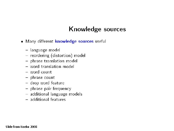
Slide from Koehn 2008

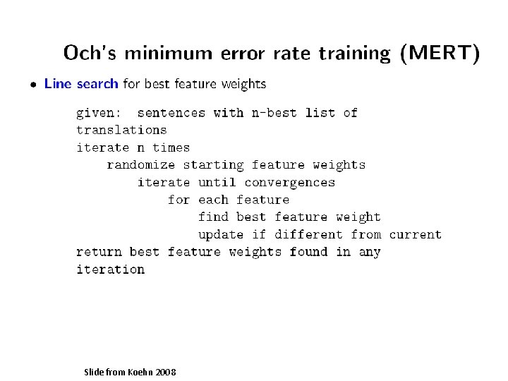
Revisiting discriminative training: methods to adjust feature weights • We will wind up with a lot of lambda scalars to optimize • But there algorithms to deal with this that are more efficient than nested for-loops • In all cases, we have the same log-linear model – The only difference is in how to optimize the lambdas – We saw one way to do this already • Using nested for-loops on n-best lists – We will keep using n-best lists (but not nested for-loops)

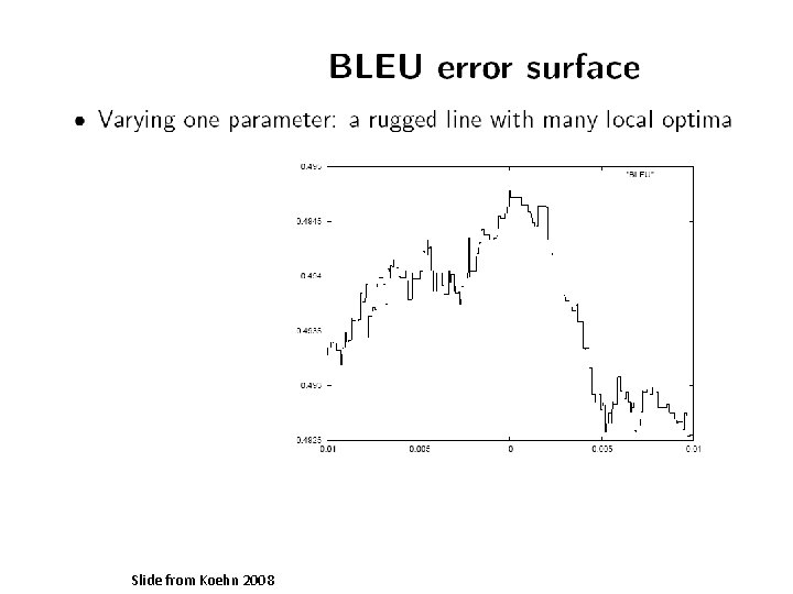
Minimum Error Rate Training – Maximize quality of top-ranked translation • Similarity according to metric (BLEU) • Implemented in Moses toolkit

Slide from Koehn 2008

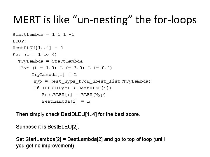
MERT is like “un-nesting” the for-loops Start. Lambda = 1 1 1 -1 LOOP: Best. BLEU[1. . 4] = 0 For (i = 1 to 4) Try. Lambda = Start. Lambda For (L = 1. 0; L <= 3. 0; L += 0. 1) Try. Lambda[i] = L Hyp = best_hyps_from_nbest_list(Try. Lambda) If (BLEU(Hyp) > Best. BLEU[i]) Best. BLEU[i] = BLEU(Hyp) Best. Lambda[i] = L Then simply check Best. BLEU[1. . 4] for the best score. Suppose it is Best. BLEU[2]. Set Start. Lambda[2] = Best. Lambda[2] and go to top of loop (until you get no improvement).

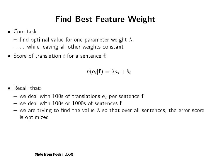
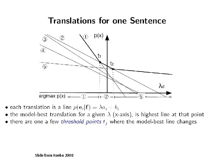
However MERT is better than that • We will not check discrete values (1. 0, 1. 1, …, 3. 0) • We will instead do an exact line minimization in one pass through the n-best list • Key observation is that varying just one weight means: – The score of each hypothesis (as we vary the weight) can be viewed as a line – For each sentence, we can look at the intercept points of these lines to see where the hypothesis with the best model score changes

Slide from Koehn 2008

Slide from Koehn 2008

Slide from Koehn 2008

Minimum Error Rate Training [Och, ACL 2003] • Maximize quality of top-ranked translation • Similarity according to metric (BLEU) • This approach only works with up to around 20 feature functions • But very fast and easy to implement • Implementation comes with Moses

Maximum Entropy [Och and Ney, ACL 2002] – Match expectation of feature values of model and reference translation – Log-linear models are also sometimes called Maximum Entropy models (when trained this way) – Great for binary classification, very many lightweight features • Also is a convex optimization – no problems with local maxima in the optimization – Doesn‘t work well for SMT

Ordinal Regression [Chiang et al. , NAACL 2009; many others previously] – Separate k worst from the k best translations • E. g. , separate hypotheses with lowest BLEU from hypotheses with highest BLEU • Approximately maximizes the margin • Support Vector machines do this non-approximately (but are too slow) • Often done in an online fashion, one sentence at a time (i. e. , original Chiang approach) • • Recently become very popular Moses comes with Batch MIRA (not online), we use this Related approach (also in Moses) is Pairwise Ranking Optimization Both approaches scale to thousands of feature functions

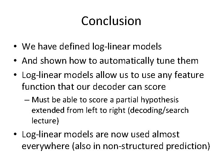
Conclusion • We have defined log-linear models • And shown how to automatically tune them • Log-linear models allow us to use any feature function that our decoder can score – Must be able to score a partial hypothesis extended from left to right (decoding/search lecture) • Log-linear models are now used almost everywhere (also in non-structured prediction)

• Thanks for your attention!

Slide from Koehn 2008