Natural Language Processing Machine Translation MT Machine translation

Natural Language Processing Machine Translation (MT)

• Machine translation was one of the first applications envisioned for computers • First demonstrated by IBM in 1954 with a basic word-for-word translation system 2

Rule-Based vs. Statistical MT • Rule-based MT: – – Hand-written transfer rules Rules can be based on lexical or structural transfer Pro: capturing complex translation phenomena Con: very labor-intensive -> lack of robustness • Statistical MT – – Mainly word or phrase-based translations Translation are learned from actual data Pro: translations are learned automatically Con: difficult to model complex translation phenomena 3

Rule-Based vs. Statistical MT • Statistical MT: Word-based Vs. Phrase-based 5

Word-Level Alignments • Given a parallel sentence pair we can align words that are translations of each other: 6

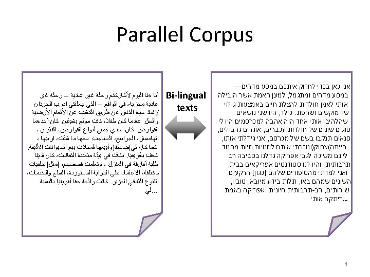
Sentence Alignment • If document De is translation of document Df how do we find the translation for each sentence? • The n-th sentence in De is not necessarily the translation of the n-th sentence in document Df • In addition to 1: 1 alignments, there also 1: 0, 0: 1, 1: n, and n: 1 alignments • Approximately 90% of the sentence alignments are 1: 1 7

Sentence Alignment (c’ntd) • There are several sentence alignment algorithms: – Align (Gale & Church): Aligns sentences based on their character length (shorter sentences tend to have shorter translations then longer sentences). Works astonishingly well – Char-align: (Church): Aligns based on shared character sequences. Works fine for similar languages or technical domains – K-Vec (Fung & Church): Induces a translation lexicon from the parallel texts based on the distribution of foreign. English word pairs. 8

Computing Translation Probabilities • Given a parallel corpus we can estimate P(e | f) • The maximum likelihood estimation of P(e | f) is: freq(e, f)/freq(f) • Way too specific to get any reasonable frequencies! Vast majority of unseen data will have zero counts! • P(e | f ) could be re-defined as: • Problem: The English words maximizing P(e | f ) might not result in a readable sentence 9

Computing Translation Probabilities (c’tnd) • We can account for adequacy: each foreign word translates into its most likely English word • We cannot guarantee that this will result in a fluent English sentence • Solution: transform P(e | f) with Bayes’ rule: P(e | f) = P(e) P(f | e) / P(f) • P(f | e) – adequacy (translation model) • P(e) – fluency (language model) 10

Decoding • The decoder combines the evidence from P(e) and P(f | e) to find the sequence e that is the best translation: 11

Noisy Channel Model for Translation 12

Translation Model • Determines the probability that the foreign word f is a translation of the English word e • How to compute P(f | e) from a parallel corpus? • Statistical approaches rely on the co-occurrence of e and f in the parallel data: If e and f tend to co-occur in parallel sentence pairs, they are likely to be translations of one another 13

Translation Steps 14

IBM Models 1– 5 • Model 1: Bag of words – Unique local maxima – Efficient EM algorithm (Model 1– 2) • Model 2: General alignment: • Model 3: fertility: n(k | e) – No full EM, count only neighbors (Model 3– 5) • Model 4: Relative distortion, word classes • Model 5: Extra variables to avoid deficiency 15

IBM Model 1 Recap • IBM Model 1 allows for an efficient computation of translation probabilities • No notion of fertility, i. e. , it’s possible that the same English word is the best translation for all foreign words • No positional information, i. e. , depending on the language pair, there might be a tendency that words occurring at the beginning of the English sentence are more likely to align to words at the beginning of the foreign sentence 16

IBM Model 3 • IBM Model 3 offers two additional features compared to IBM Model 1: – How likely is an English word e to align to k foreign words (fertility)? – Positional information (distortion), how likely is a word in position i to align to a word in position j? 17

IBM Model 3: Fertility • The best Model 1 alignment could be that a single English word aligns to all foreign words • This is clearly not desirable and we want to constrain the number of words an English word can align to • Fertility models a probability distribution that word e aligns to k words: n(k, e) • Consequence: translation probabilities cannot be computed independently of each other anymore • IBM Model 3 has to work with full alignments, note there are up to (l+1)m different alignments 18

IBM Model 1 + Model 3 • Iterating over all possible alignments is computationally infeasible • Solution: Compute the best alignment with Model 1 and change some of the alignments to generate a set of likely alignments (pegging) • Model 3 takes this restricted set of alignments as input 19

Pegging • Given an alignment a we can derive additional alignments from it by making small changes: – Changing a link (j, i) to (j, i’) – Swapping a pair of links (j, i) and (j’, i’) to (j, i’) and (j’, i) • The resulting set of alignments is called the neighborhood of a 20

IBM Model 3: Distortion • The distortion factor determines how likely it is that an English word in position i aligns to a foreign word in position j, given the lengths of both sentences: d(j | i, l, m) • Note, positions are absolute positions 21

Deficiency • Problem with IBM Model 3: It assigns probability mass to impossible strings – Well formed string: “This is possible” – Ill-formed but possible string: “This possible is” – Impossible string: • Impossible strings are due to distortion values that generate different words at the same position • Impossible strings can still be filtered out in later stages of the translation process 22

Limitations of IBM Models • Only 1 -to-N word mapping • Handling fertility-zero words (difficult for decoding) • Almost no syntactic information – Word classes – Relative distortion • Long-distance word movement • Fluency of the output depends entirely on the English language model 23

Phrase-based models • Word-based models translate words as atomic units • Phrase-based models translate phases as atomic units

Phrase Table • Main knowledge source: table with phrase translations and their probabilities • Example for natuerlich

Learning a Phrase Table • From a parallel corpus: – First run word alignment – Then, extract phrases – Finally assign phrase probabilities

Extract Phrases • Extract consistent phrases

Extract Phrases

Consistent Phrase

Assign Phrase Probabilities

Phrase-based Model

Log-linear model