Smoothing Techniques A Primer Deepak Suyel Geetanjali Rakshit

Smoothing Techniques – A Primer Deepak Suyel Geetanjali Rakshit Sachin Pawar CS 626 – Speech, NLP and the Web 02 -Nov-12 1

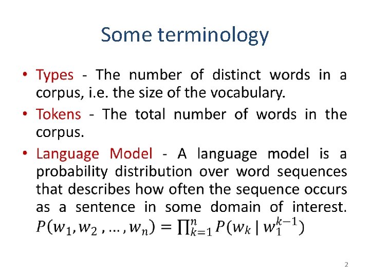
Some terminology • 2

Language Models • Language models are useful for NLP applications such as – Next word prediction – Machine translation – Spelling correction – Authorship Identification – Natural language generation • For intrinsic evaluation of language models, Perplexity metric is used. 3

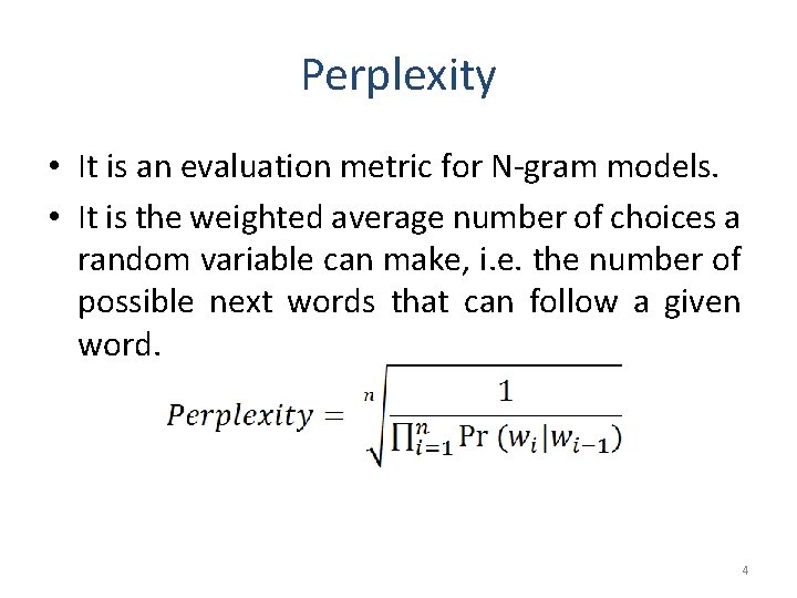
Perplexity • It is an evaluation metric for N-gram models. • It is the weighted average number of choices a random variable can make, i. e. the number of possible next words that can follow a given word. 4

Roadmap • • • Motivation Types of smoothing Back-off Interpolation Comparison of smoothing techniques 5

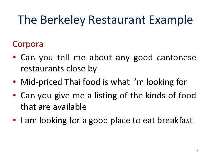
The Berkeley Restaurant Example Corpora • Can you tell me about any good cantonese restaurants close by • Mid-priced Thai food is what I’m looking for • Can you give me a listing of the kinds of food that are available • I am looking for a good place to eat breakfast 6

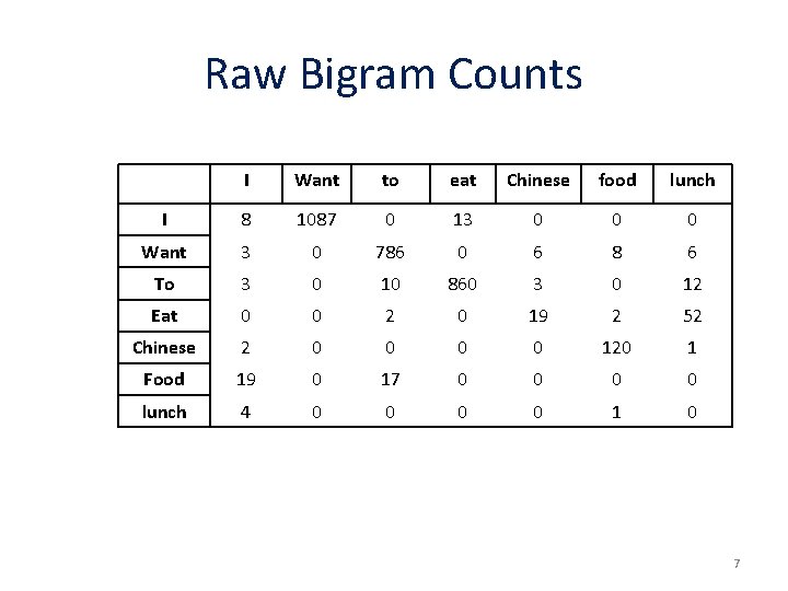
Raw Bigram Counts I Want to eat Chinese food lunch I 8 1087 0 13 0 0 0 Want 3 0 786 0 6 8 6 To 3 0 10 860 3 0 12 Eat 0 0 2 0 19 2 52 Chinese 2 0 0 120 1 Food 19 0 17 0 0 lunch 4 0 0 1 0 7

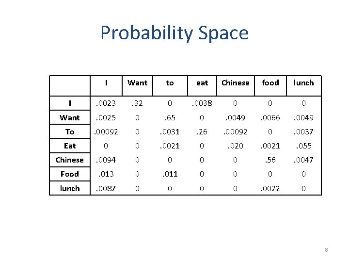
Probability Space I Want to eat Chinese food lunch I . 0023 . 32 0 . 0038 0 0 0 Want . 0025 0 . 65 0 . 0049 . 0066 . 0049 To . 00092 0 . 0031 . 26 . 00092 0 . 0037 Eat 0 0 . 0021 0 . 020 . 0021 . 055 Chinese . 0094 0 0 . 56 . 0047 Food . 013 0 . 011 0 0 lunch . 0087 0 0 . 0022 0 8

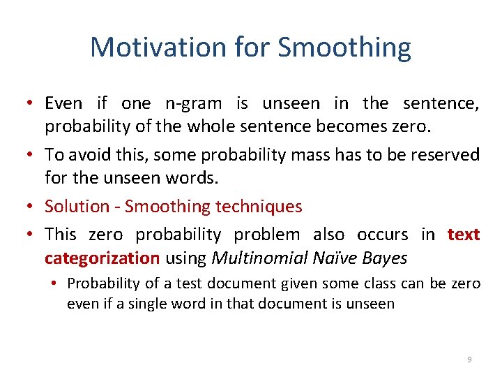
Motivation for Smoothing • Even if one n-gram is unseen in the sentence, probability of the whole sentence becomes zero. • To avoid this, some probability mass has to be reserved for the unseen words. • Solution - Smoothing techniques • This zero probability problem also occurs in text categorization using Multinomial Naïve Bayes • Probability of a test document given some class can be zero even if a single word in that document is unseen 9

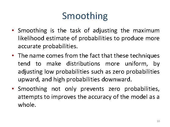
Smoothing • Smoothing is the task of adjusting the maximum likelihood estimate of probabilities to produce more accurate probabilities. • The name comes from the fact that these techniques tend to make distributions more uniform, by adjusting low probabilities such as zero probabilities upward, and high probabilities downward. • Smoothing not only prevents zero probabilities, attempts to improves the accuracy of the model as a whole. 10

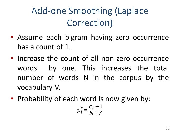
Add-one Smoothing (Laplace Correction) • 11

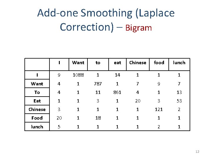
Add-one Smoothing (Laplace Correction) – Bigram I Want to eat Chinese food lunch I 9 1088 1 14 1 1 1 Want 4 1 787 1 7 9 7 To 4 1 11 861 4 1 13 Eat 1 1 3 1 20 3 53 Chinese 3 1 1 121 2 Food 20 1 18 1 1 lunch 5 1 1 2 1 12

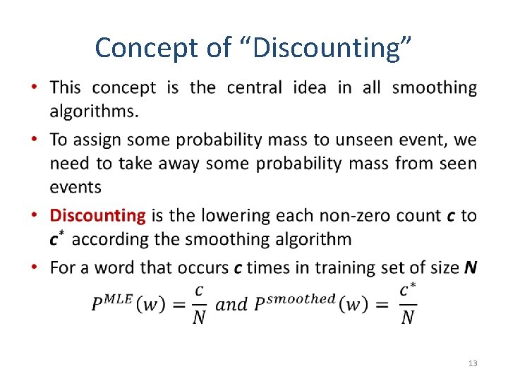
Concept of “Discounting” • 13

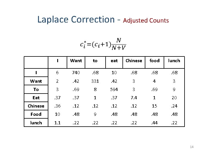
Laplace Correction - Adjusted Counts • I Want to eat Chinese food lunch I 6 740 . 68 10 . 68 Want 2 . 42 331 . 42 3 4 3 To 3 . 69 8 594 3 . 69 9 Eat . 37 1 . 37 7. 4 1 20 Chinese . 36 . 12 15 . 24 Food 10 . 48 9 . 48 lunch 1. 1 . 22 . 44 . 22 14

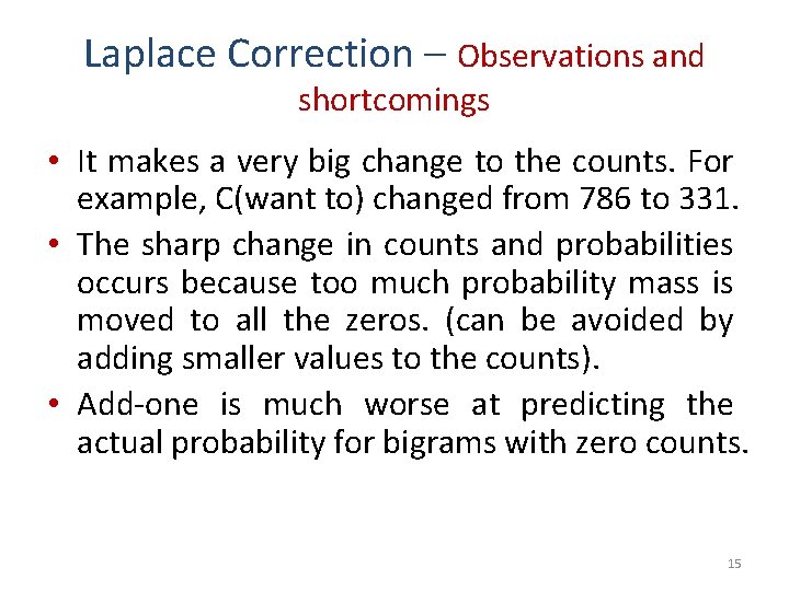
Laplace Correction – Observations and shortcomings • It makes a very big change to the counts. For example, C(want to) changed from 786 to 331. • The sharp change in counts and probabilities occurs because too much probability mass is moved to all the zeros. (can be avoided by adding smaller values to the counts). • Add-one is much worse at predicting the actual probability for bigrams with zero counts. 15

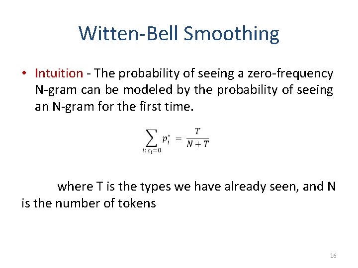
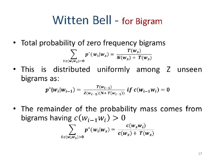
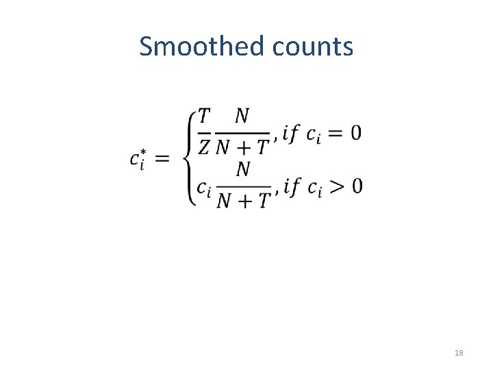
Witten-Bell Smoothing • Intuition - The probability of seeing a zero-frequency N-gram can be modeled by the probability of seeing an N-gram for the first time. where T is the types we have already seen, and N is the number of tokens 16

Witten Bell - for Bigram • 17

Smoothed counts • 18

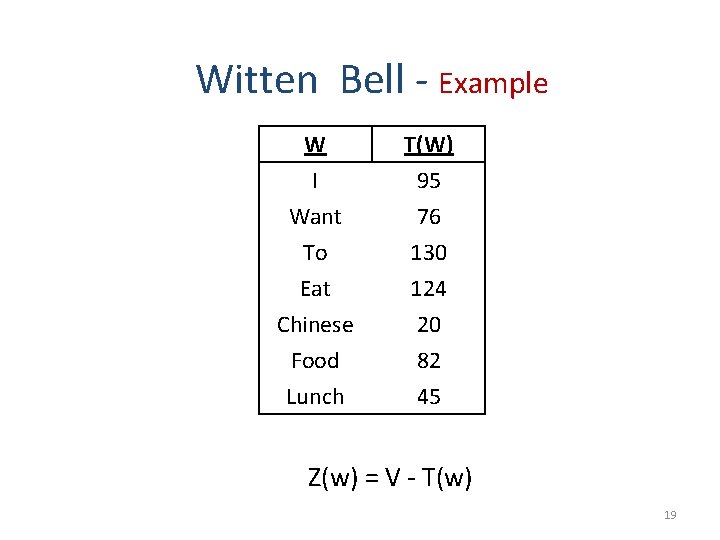
Witten Bell - Example W I Want To T(W) 95 76 130 Eat Chinese Food Lunch 124 20 82 45 Z(w) = V - T(w) 19

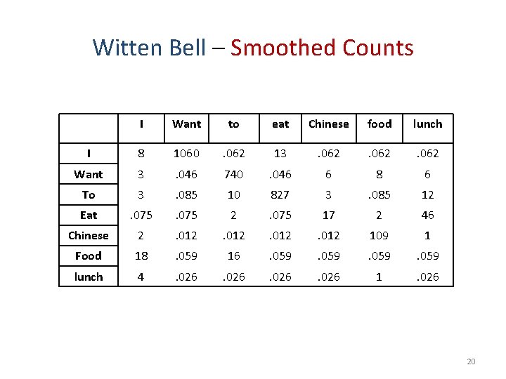
Witten Bell – Smoothed Counts I Want to eat Chinese food lunch I 8 1060 . 062 13 . 062 Want 3 . 046 740 . 046 6 8 6 To 3 . 085 10 827 3 . 085 12 Eat . 075 2 . 075 17 2 46 Chinese 2 . 012 109 1 Food 18 . 059 16 . 059 lunch 4 . 026 1 . 026 20

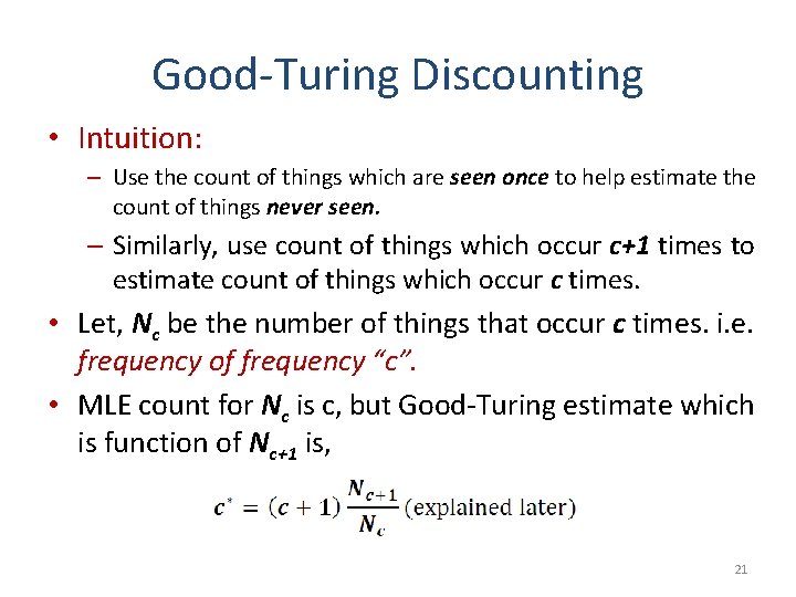
Good-Turing Discounting • Intuition: – Use the count of things which are seen once to help estimate the count of things never seen. – Similarly, use count of things which occur c+1 times to estimate count of things which occur c times. • Let, Nc be the number of things that occur c times. i. e. frequency of frequency “c”. • MLE count for Nc is c, but Good-Turing estimate which is function of Nc+1 is, 21

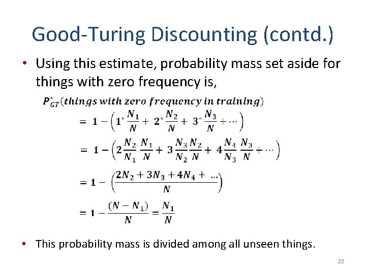
Good-Turing Discounting (contd. ) • Using this estimate, probability mass set aside for things with zero frequency is, • This probability mass is divided among all unseen things. 22

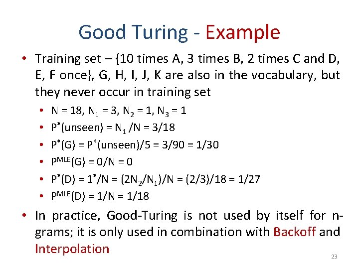
Good Turing - Example • Training set – {10 times A, 3 times B, 2 times C and D, E, F once}, G, H, I, J, K are also in the vocabulary, but they never occur in training set • • • N = 18, N 1 = 3, N 2 = 1, N 3 = 1 P*(unseen) = N 1 /N = 3/18 P*(G) = P*(unseen)/5 = 3/90 = 1/30 PMLE(G) = 0/N = 0 P*(D) = 1*/N = (2 N 2/N 1)/N = (2/3)/18 = 1/27 PMLE(D) = 1/N = 1/18 • In practice, Good-Turing is not used by itself for ngrams; it is only used in combination with Backoff and Interpolation 23

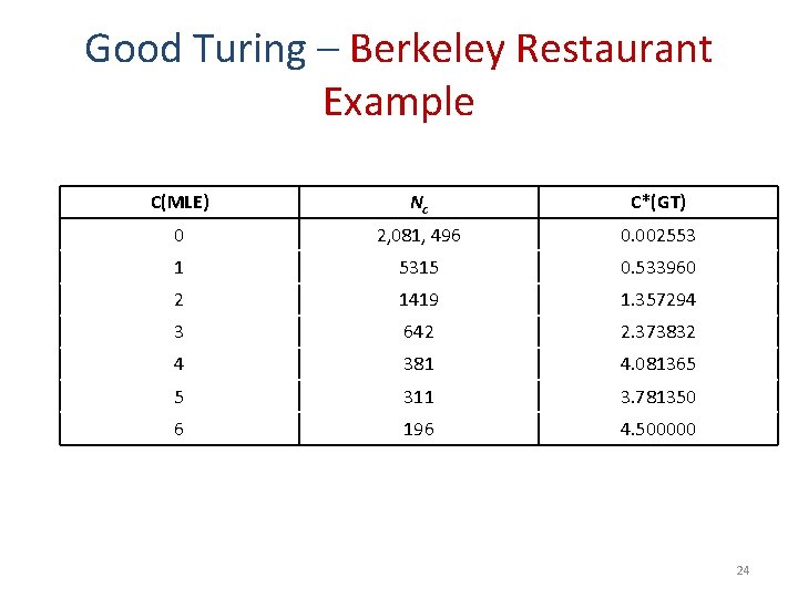
Good Turing – Berkeley Restaurant Example C(MLE) Nc C*(GT) 0 2, 081, 496 0. 002553 1 5315 0. 533960 2 1419 1. 357294 3 642 2. 373832 4 381 4. 081365 5 311 3. 781350 6 196 4. 500000 24

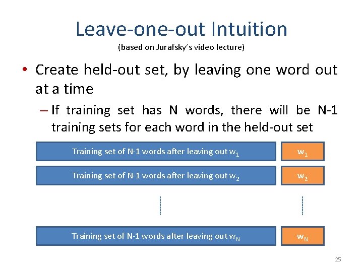
Leave-one-out Intuition (based on Jurafsky’s video lecture) • Create held-out set, by leaving one word out at a time – If training set has N words, there will be N-1 training sets for each word in the held-out set Training set of N-1 words after leaving out w 1 Training set of N-1 words after leaving out w 2 Training set of N-1 words after leaving out w. N 25

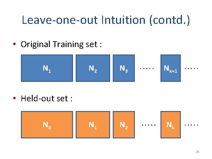
Leave-one-out Intuition (contd. ) • Original Training set : N 1 N 2 N 3 Nk+1 Nk • Held-out set : N 0 N 1 N 2 26

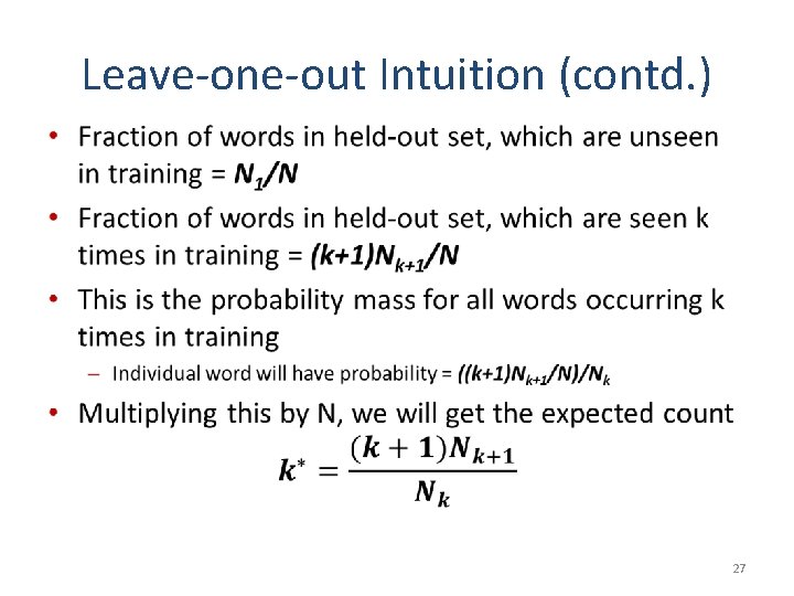
Leave-one-out Intuition (contd. ) • 27

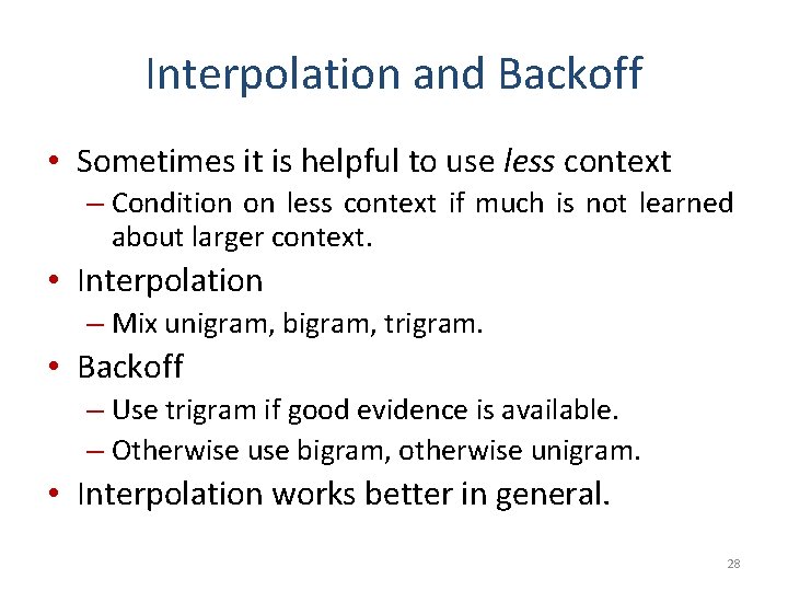
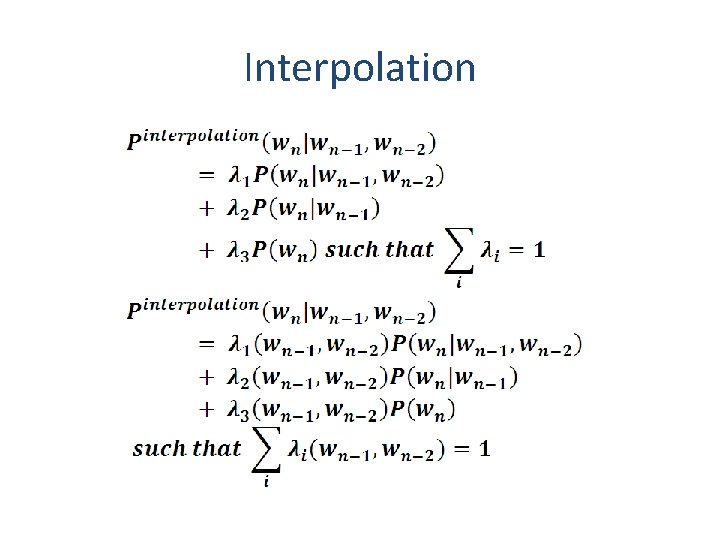
Interpolation and Backoff • Sometimes it is helpful to use less context – Condition on less context if much is not learned about larger context. • Interpolation – Mix unigram, bigram, trigram. • Backoff – Use trigram if good evidence is available. – Otherwise use bigram, otherwise unigram. • Interpolation works better in general. 28

Interpolation

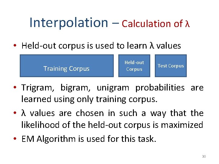
Interpolation – Calculation of λ • Held-out corpus is used to learn λ values Training Corpus Held-out Corpus Test Corpus • Trigram, bigram, unigram probabilities are learned using only training corpus. • λ values are chosen in such a way that the likelihood of the held-out corpus is maximized • EM Algorithm is used for this task. 30

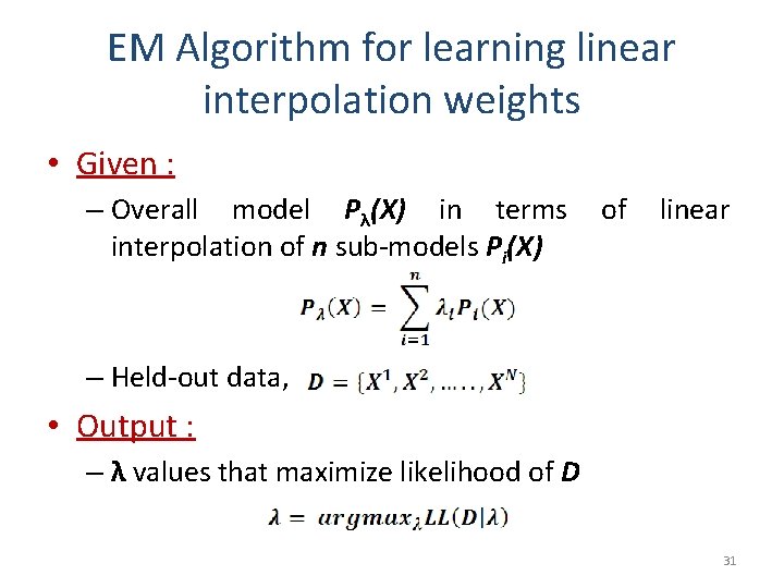
EM Algorithm for learning linear interpolation weights • Given : – Overall model Pλ(X) in terms of linear interpolation of n sub-models Pi(X) – Held-out data, • Output : – λ values that maximize likelihood of D 31

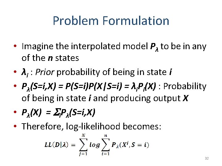
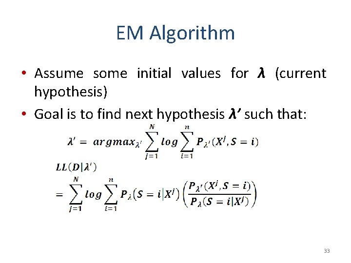
Problem Formulation • Imagine the interpolated model Pλ to be in any of the n states • λi : Prior probability of being in state i • Pλ(S=i, X) = P(S=i)P(X|S=i) = λi. Pi(X) : Probability of being in state i and producing output X • Pλ(X) = i. Pλ(S=i, X) • Therefore, log-likelihood becomes: 32

EM Algorithm • Assume some initial values for λ (current hypothesis) • Goal is to find next hypothesis λ’ such that: 33

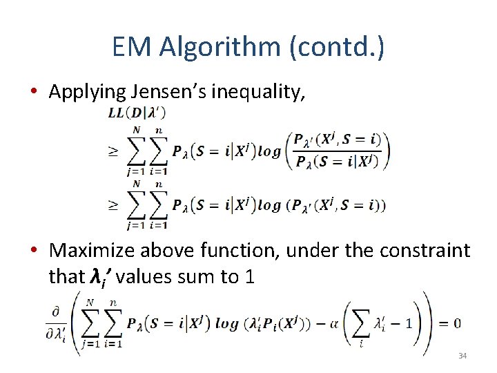
EM Algorithm (contd. ) • Applying Jensen’s inequality, • Maximize above function, under the constraint that λi’ values sum to 1 34

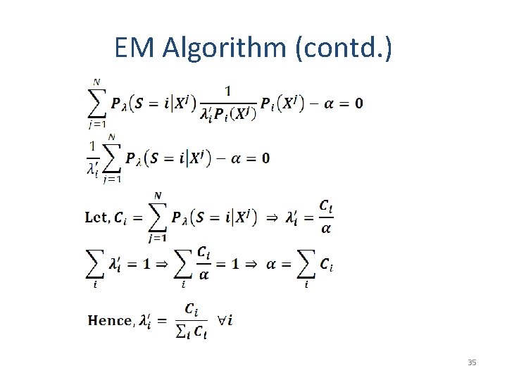
EM Algorithm (contd. ) 35

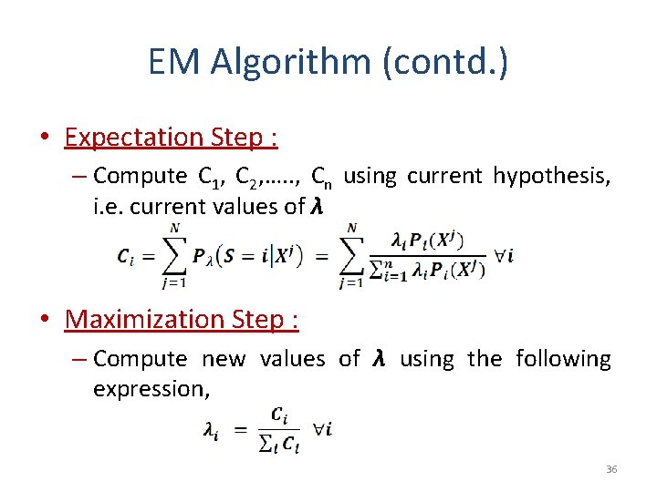
EM Algorithm (contd. ) • Expectation Step : – Compute C 1, C 2, …. . , Cn using current hypothesis, i. e. current values of λ • Maximization Step : – Compute new values of λ using the following expression, 36

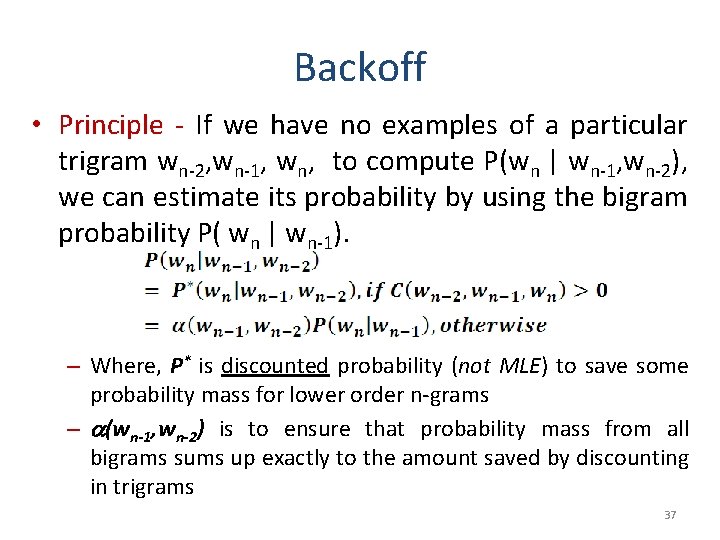
Backoff • Principle - If we have no examples of a particular trigram wn-2, wn-1, wn, to compute P(wn | wn-1, wn-2), we can estimate its probability by using the bigram probability P( wn | wn-1). – Where, P* is discounted probability (not MLE) to save some probability mass for lower order n-grams – (wn-1, wn-2) is to ensure that probability mass from all bigrams sums up exactly to the amount saved by discounting in trigrams 37

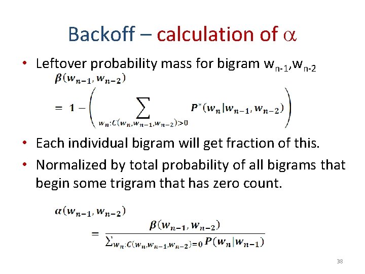
Backoff – calculation of • Leftover probability mass for bigram wn-1, wn-2 • Each individual bigram will get fraction of this. • Normalized by total probability of all bigrams that begin some trigram that has zero count. 38

Stupid Backoff (contd. ) • Authors named this method stupid, because their initial thought was that such a simple scheme can’t be possibly good. • But this method turned out to be as good as the state of the art “Kneser Ney”. (discussed later) • Important conclusions: – Inexpensive calculations, but quite accurate if training set is large. – Lack of normalization doesn’t affect, because functioning of LM in their setting depends on relative rather than absolute scores.

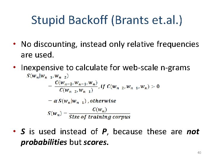
Stupid Backoff (Brants et. al. ) • No discounting, instead only relative frequencies are used. • Inexpensive to calculate for web-scale n-grams • S is used instead of P, because these are not probabilities but scores. 40

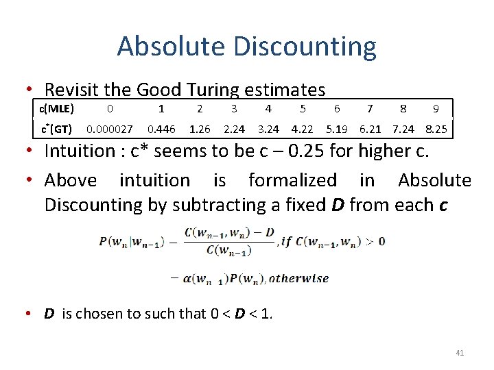
Absolute Discounting • Revisit the Good Turing estimates c(MLE) 0 1 2 3 4 c*(GT) 0. 000027 0. 446 1. 26 2. 24 3. 24 5 6 7 8 9 4. 22 5. 19 6. 21 7. 24 8. 25 • Intuition : c* seems to be c – 0. 25 for higher c. • Above intuition is formalized in Absolute Discounting by subtracting a fixed D from each c • D is chosen to such that 0 < D < 1. 41

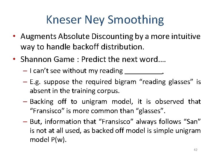
Kneser Ney Smoothing • Augments Absolute Discounting by a more intuitive way to handle backoff distribution. • Shannon Game : Predict the next word…. – I can’t see without my reading . – E. g. suppose the required bigram “reading glasses” is absent in the training corpus. – Backing off to unigram model, it is observed that “Fransisco” is more common than “glasses”. – But, information that “Fransisco” always follows “San” is not at all used, as backed off model is simple unigram model P(w). 42

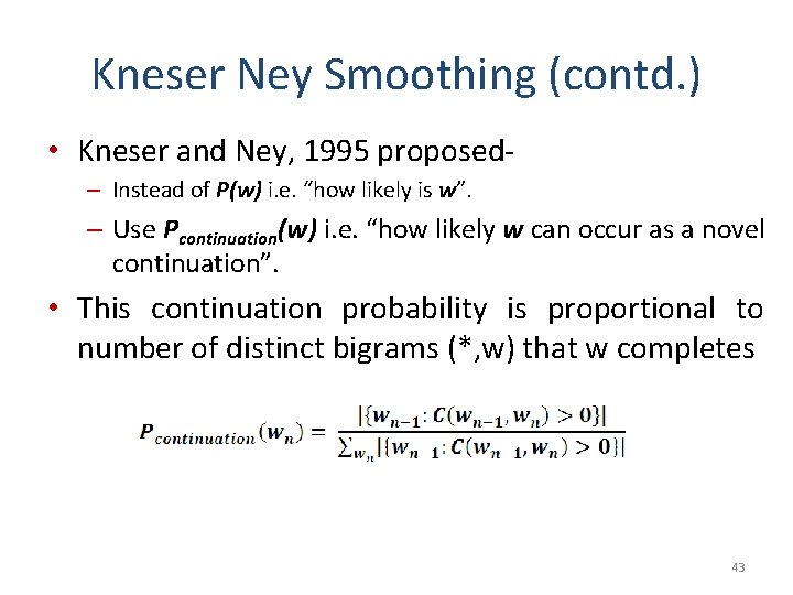
Kneser Ney Smoothing (contd. ) • Kneser and Ney, 1995 proposed– Instead of P(w) i. e. “how likely is w”. – Use Pcontinuation(w) i. e. “how likely w can occur as a novel continuation”. • This continuation probability is proportional to number of distinct bigrams (*, w) that w completes 43

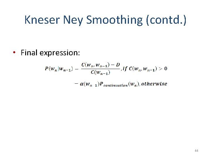
Kneser Ney Smoothing (contd. ) • Final expression: 44

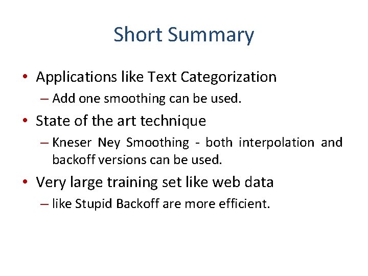
Short Summary • Applications like Text Categorization – Add one smoothing can be used. • State of the art technique – Kneser Ney Smoothing - both interpolation and backoff versions can be used. • Very large training set like web data – like Stupid Backoff are more efficient.

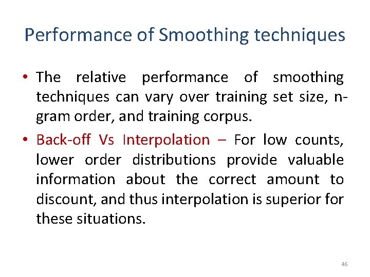
Performance of Smoothing techniques • The relative performance of smoothing techniques can vary over training set size, ngram order, and training corpus. • Back-off Vs Interpolation – For low counts, lower order distributions provide valuable information about the correct amount to discount, and thus interpolation is superior for these situations. 46

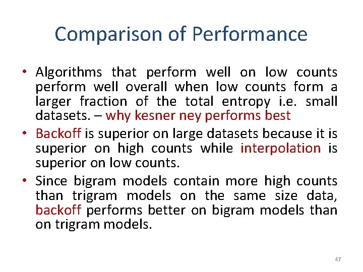
Comparison of Performance • Algorithms that perform well on low counts perform well overall when low counts form a larger fraction of the total entropy i. e. small datasets. – why kesner ney performs best • Backoff is superior on large datasets because it is superior on high counts while interpolation is superior on low counts. • Since bigram models contain more high counts than trigram models on the same size data, backoff performs better on bigram models than on trigram models. 47

Summary • Need for Smoothing • Types of smoothing – Laplace Correction – Witten Bell – Good Turing – Kesner Ney • Backoff – Back off – Interpolation • Comparison 48

References • SF Chen, J Goodman , An empirical study of smoothing techniques for language modeling- Computer Speech & Language, 1999 • Jurafsky, Daniel, and James H. Martin. 2009. Speech and Language Processing: An Introduction to Natural Language Processing, Speech Recognition, and Computational Linguistics. 2 nd edition. Prentice-Hall. • H Ney, U Essen, R Kneser, On the estimation of `small' probabilities by leaving-one-out, Pattern Analysis and Machine Intelligence, 1995 • T Brants, AC Popat, P Xu, FJ Och, J Dean, Large language models in machine translation, EMNLP 2007 • Adam Berger, Convexity, Maximum Likelihood and All That, Tutorial at http: //www. cs. cmu. edu/~aberger/maxent. html • Jurafsky’s video lecture on Language Modelling : http: //www. youtube. com/watch? v=Xdj. CCk. FUBKU 49