Signal processing Example data Ch IPSeq T N

Signal processing

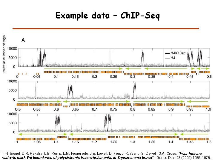
Example data – Ch. IP-Seq T. N. Siegel, D. R. Hekstra, L. E. Kemp, L. M. Figueiredo, J. E. Lowell, D. Fenyö, X. Wang, S. Dewell, G. A. Cross, "Four histone variants mark the boundaries of polycistronic transcription units in Trypanosoma brucei", Genes Dev. 23 (2009) 1063 -1076.

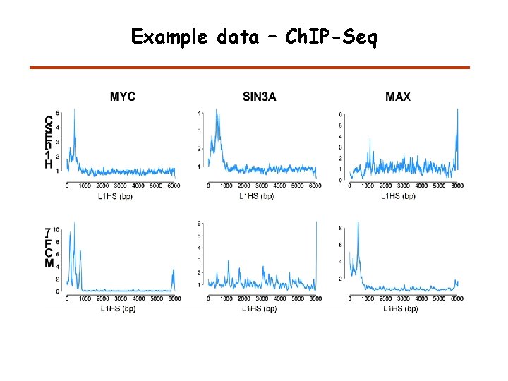
Example data – Ch. IP-Seq

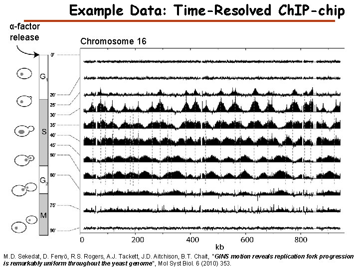
Example Data: Time-Resolved Ch. IP-chip α-factor release Chromosome 16 M. D. Sekedat, D. Fenyö, R. S. Rogers, A. J. Tackett, J. D. Aitchison, B. T. Chait, "GINS motion reveals replication fork progression is remarkably uniform throughout the yeast genome", Mol Syst Biol. 6 (2010) 353.

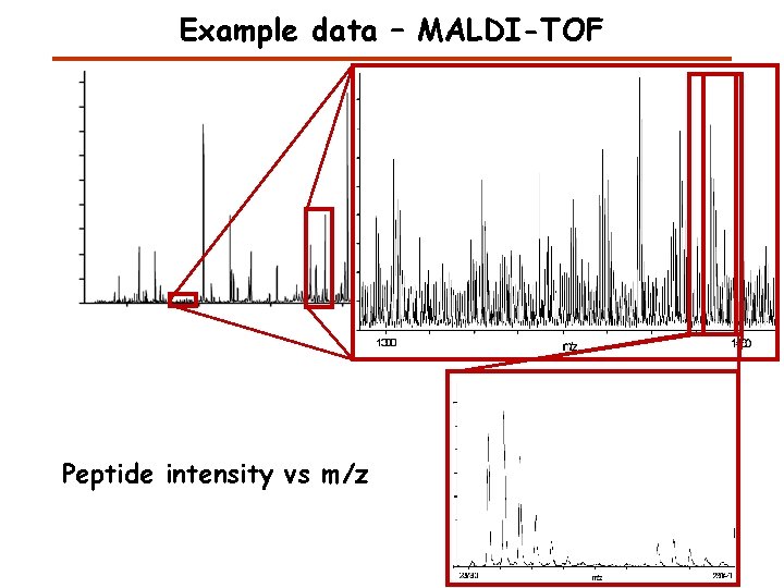
Example data – MALDI-TOF Peptide intensity vs m/z

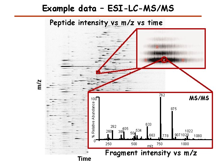
Example data – ESI-LC-MS/MS m/z Peptide intensity vs m/z vs time 762 % Relative Abundance 100 0 Time MS/MS 875 [M+2 H]2+ 292 405 534 260 389 504 250 500 633 663 m/z 778 750 1022 9071020 1080 1000 Fragment intensity vs m/z

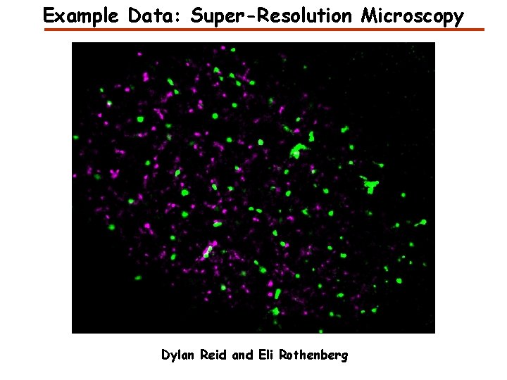
Example Data: Super-Resolution Microscopy Dylan Reid and Eli Rothenberg

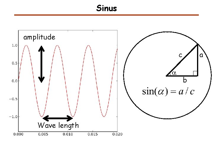
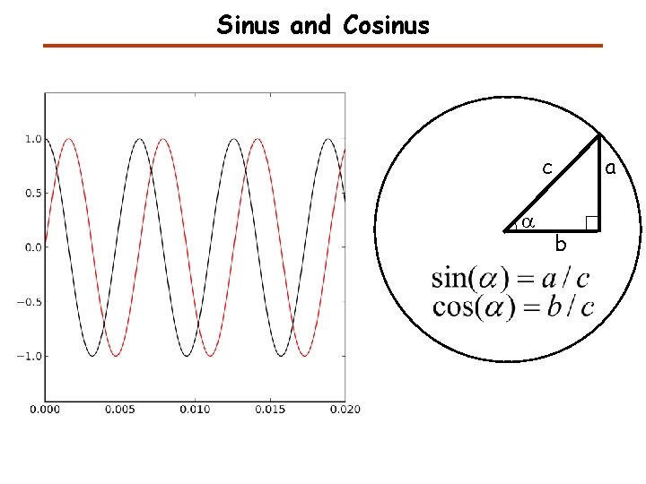
Sinus amplitude c a Wave length a b

Sinus and Cosinus c a a b

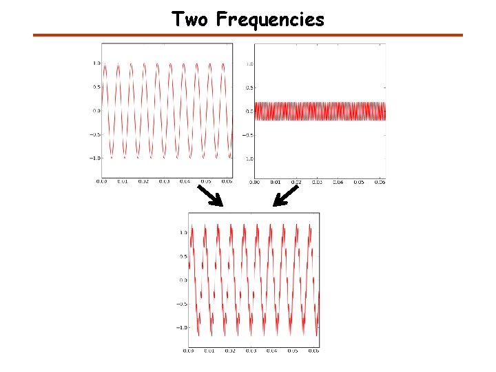
Two Frequencies

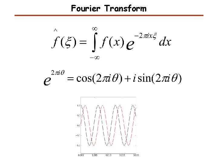
Fourier Transform

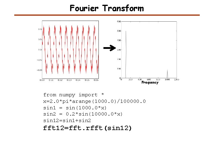
Fourier Transform Frequency from numpy import * x=2. 0*pi*arange(1000. 0)/100000. 0 sin 1 = sin(1000. 0*x) sin 2 = 0. 2*sin(10000. 0*x) sin 12=sin 1+sin 2 fft 12=fft. rfft(sin 12)

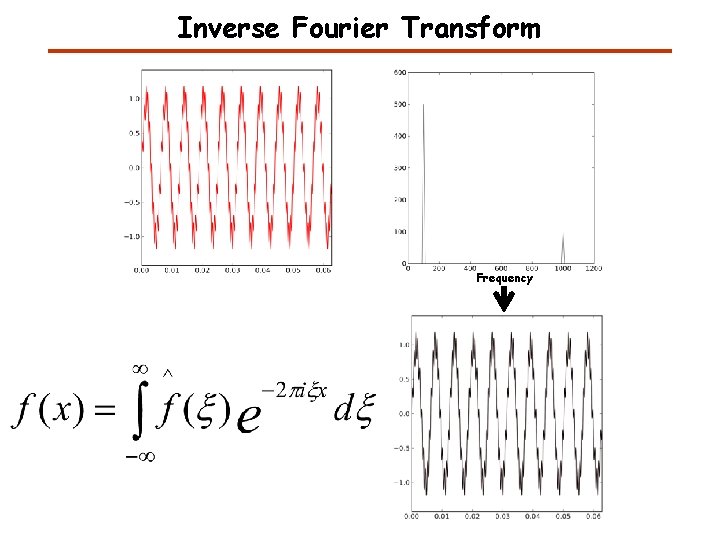
Inverse Fourier Transform Frequency

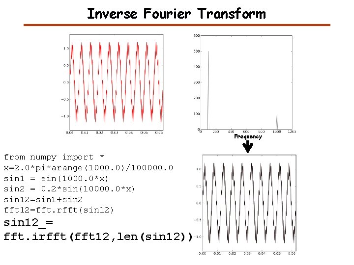
Inverse Fourier Transform Frequency from numpy import * x=2. 0*pi*arange(1000. 0)/100000. 0 sin 1 = sin(1000. 0*x) sin 2 = 0. 2*sin(10000. 0*x) sin 12=sin 1+sin 2 fft 12=fft. rfft(sin 12) sin 12_= fft. irfft(fft 12, len(sin 12))

Inverse Fourier Transform Frequency

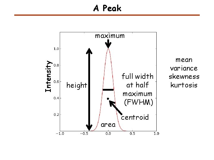
A Peak Intensity maximum full width at half maximum (FWHM) height area centroid mean variance skewness kurtosis

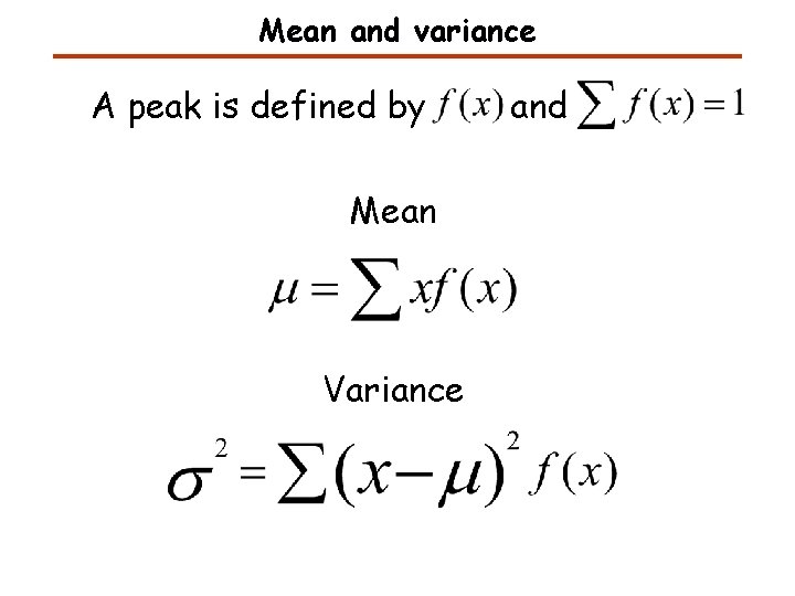
Mean and variance A peak is defined by Mean Variance and

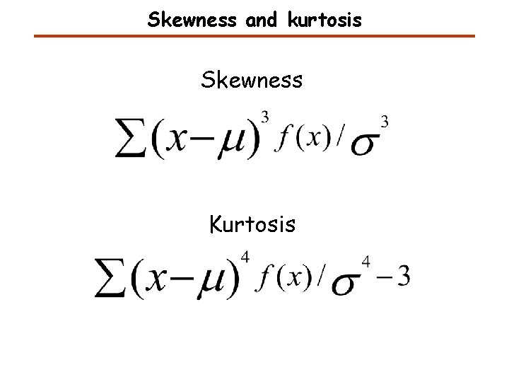
Skewness and kurtosis Skewness Kurtosis

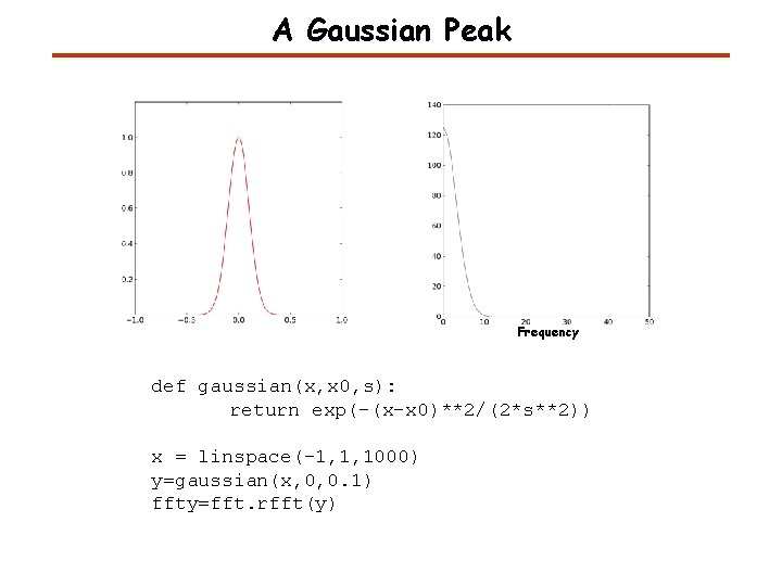
A Gaussian Peak Frequency def gaussian(x, x 0, s): return exp(-(x-x 0)**2/(2*s**2)) x = linspace(-1, 1, 1000) y=gaussian(x, 0, 0. 1) ffty=fft. rfft(y)

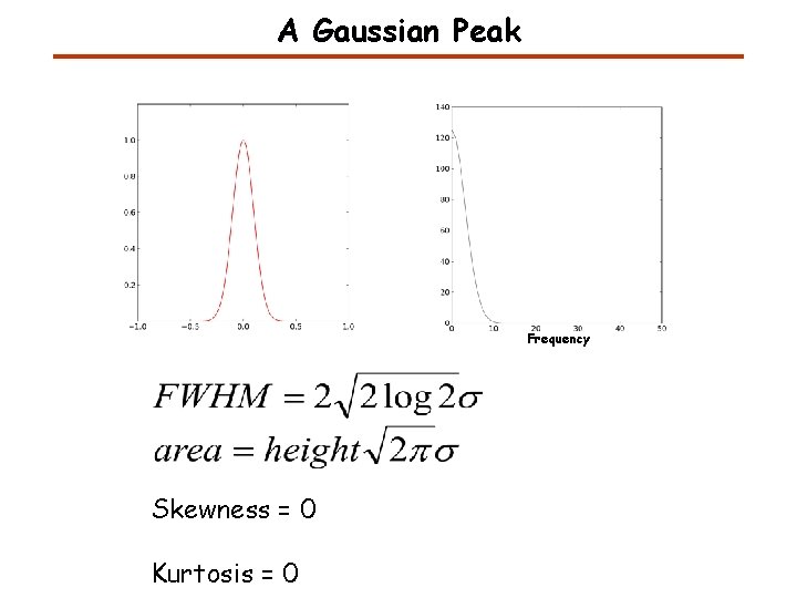
A Gaussian Peak Frequency Skewness = 0 Kurtosis = 0

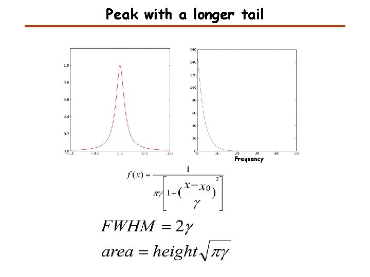
Peak with a longer tail Frequency

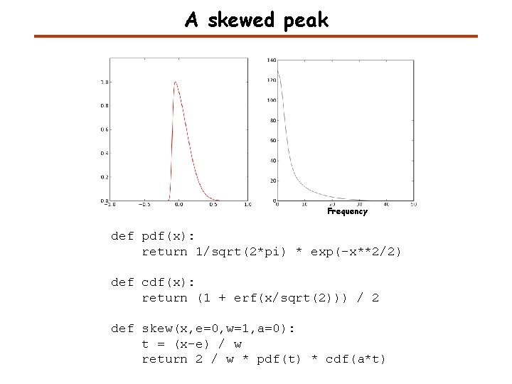
A skewed peak Frequency def pdf(x): return 1/sqrt(2*pi) * exp(-x**2/2) def cdf(x): return (1 + erf(x/sqrt(2))) / 2 def skew(x, e=0, w=1, a=0): t = (x-e) / w return 2 / w * pdf(t) * cdf(a*t)

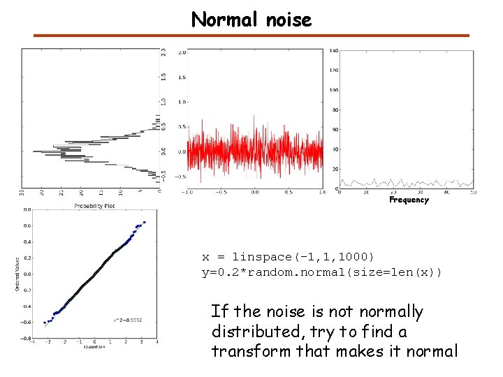
Normal noise Frequency x = linspace(-1, 1, 1000) y=0. 2*random. normal(size=len(x)) If the noise is not normally distributed, try to find a transform that makes it normal

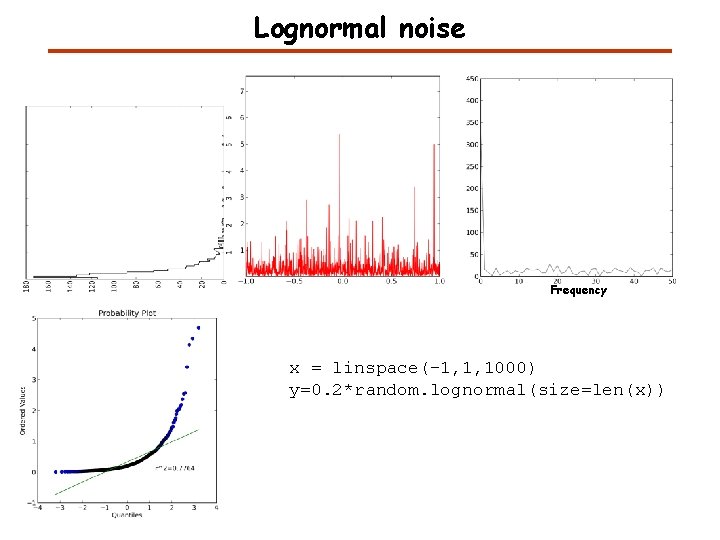
Lognormal noise Frequency x = linspace(-1, 1, 1000) y=0. 2*random. lognormal(size=len(x))

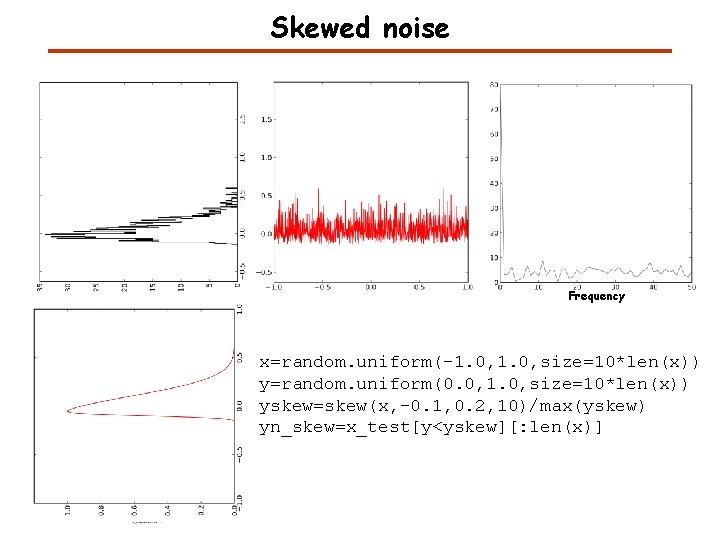
Skewed noise Frequency x=random. uniform(-1. 0, size=10*len(x)) y=random. uniform(0. 0, 1. 0, size=10*len(x)) yskew=skew(x, -0. 1, 0. 2, 10)/max(yskew) yn_skew=x_test[y<yskew][: len(x)]

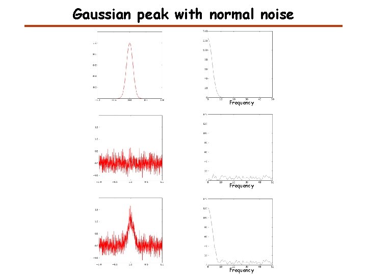
Gaussian peak with normal noise Frequency

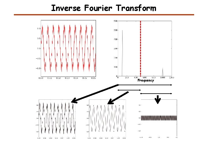
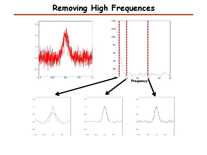
Removing High Frequences Frequency

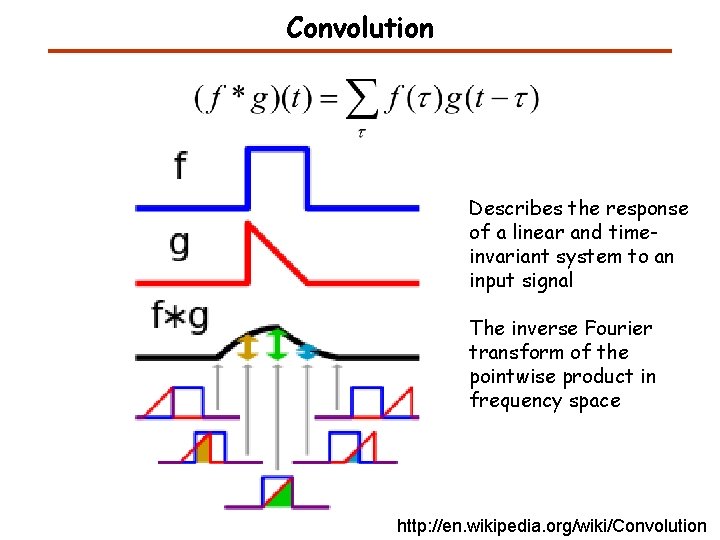
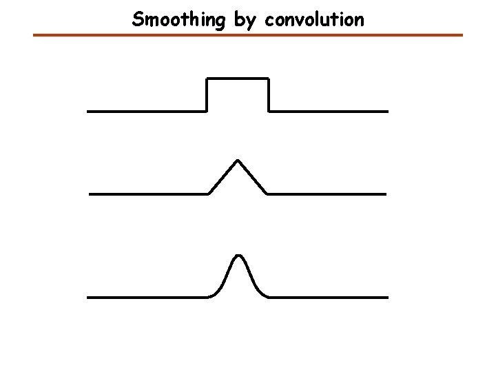
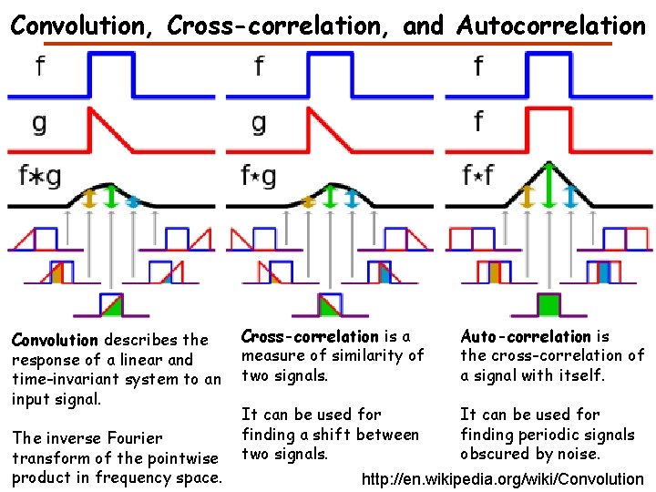
Convolution Describes the response of a linear and timeinvariant system to an input signal The inverse Fourier transform of the pointwise product in frequency space http: //en. wikipedia. org/wiki/Convolution

Smoothing by convolution

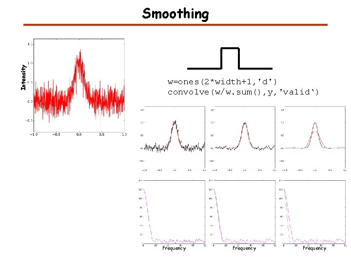
Intensity Smoothing w=ones(2*width+1, 'd') convolve(w/w. sum(), y, 'valid‘) Frequency

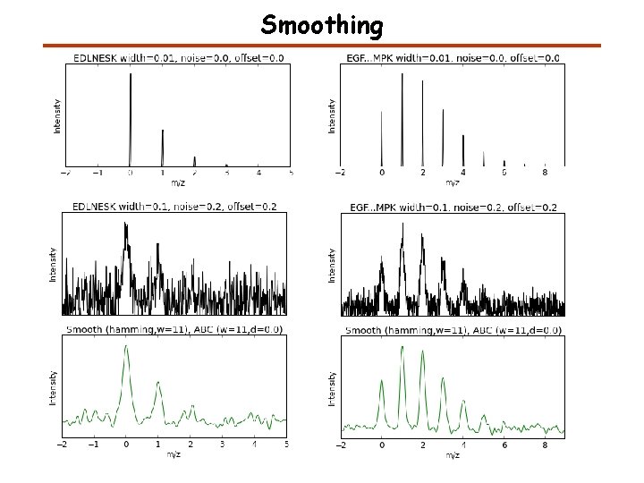
Smoothing

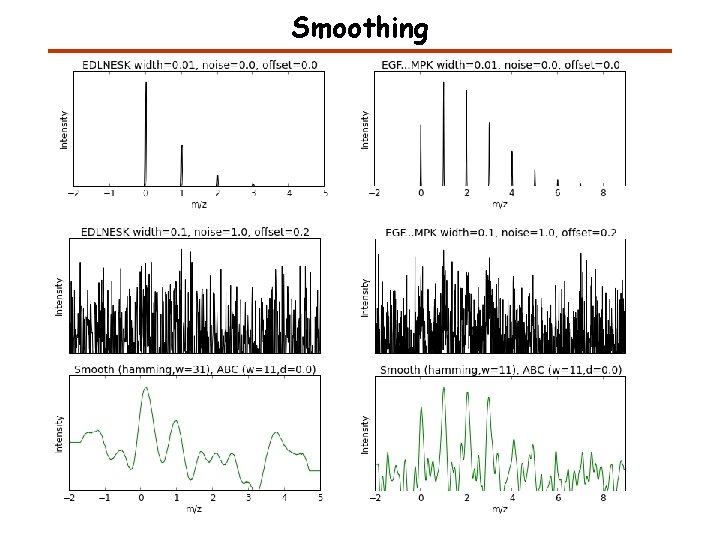
Smoothing

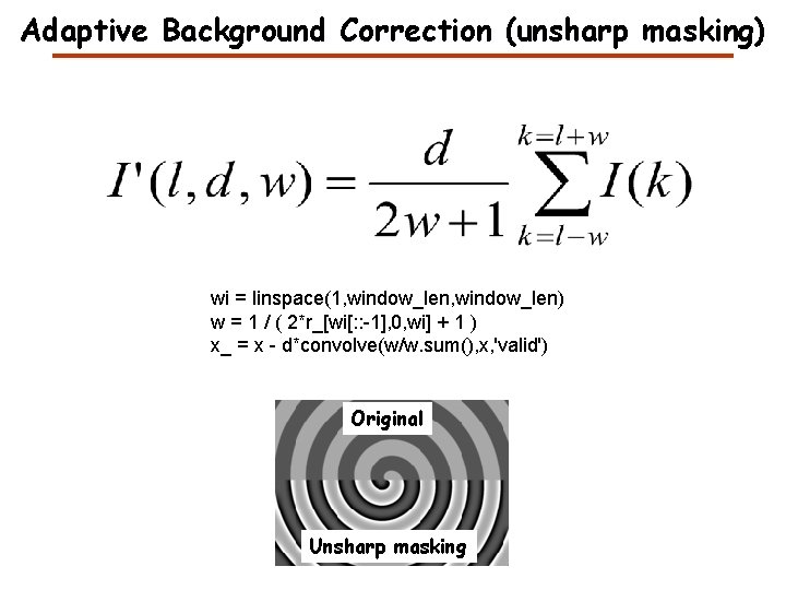
Adaptive Background Correction (unsharp masking) wi = linspace(1, window_len) w = 1 / ( 2*r_[wi[: : -1], 0, wi] + 1 ) x_ = x - d*convolve(w/w. sum(), x, 'valid') Original Unsharp masking

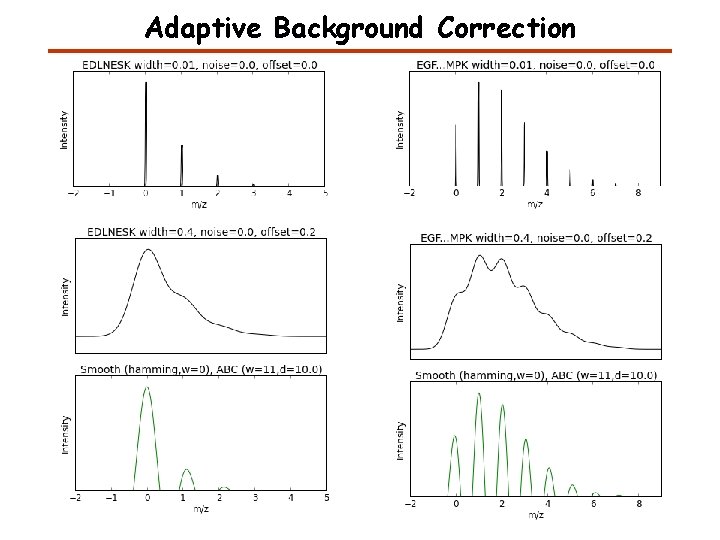
Adaptive Background Correction

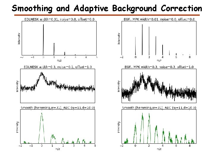
Smoothing and Adaptive Background Correction

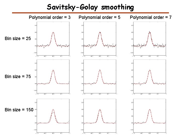
Savitsky-Golay smoothing Polynomial order = 3 Bin size = 25 Bin size = 75 Bin size = 150 Polynomial order = 5 Polynomial order = 7

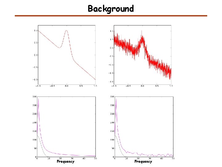
Background Frequency

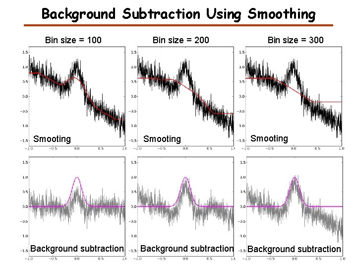
Background Subtraction Using Smoothing Bin size = 100 Smooting Background subtraction Bin size = 200 Smooting Background subtraction Bin size = 300 Smooting Background subtraction

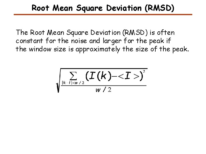
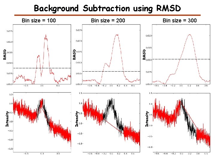
Root Mean Square Deviation (RMSD) The Root Mean Square Deviation (RMSD) is often constant for the noise and larger for the peak if the window size is approximately the size of the peak.

Background Subtraction using RMSD Bin size = 300 Intensity RMSD Bin size = 200 Intensity RMSD Bin size = 100

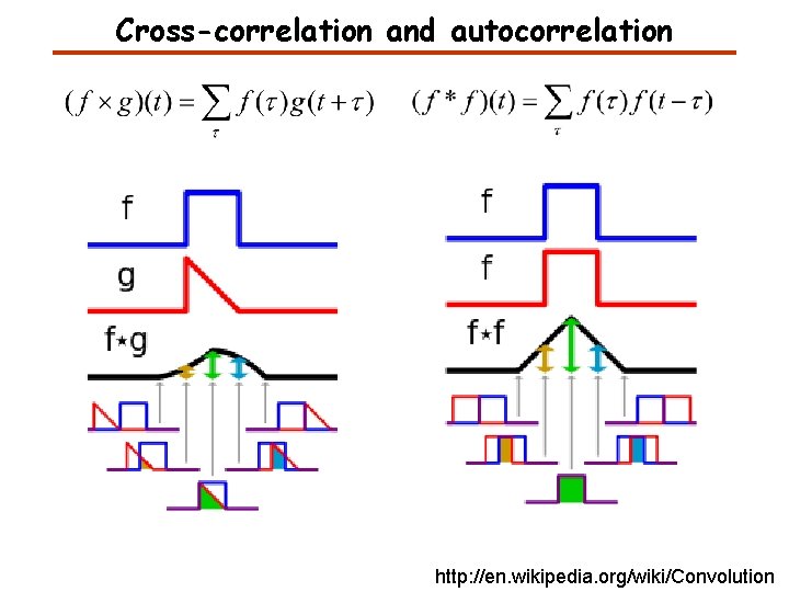
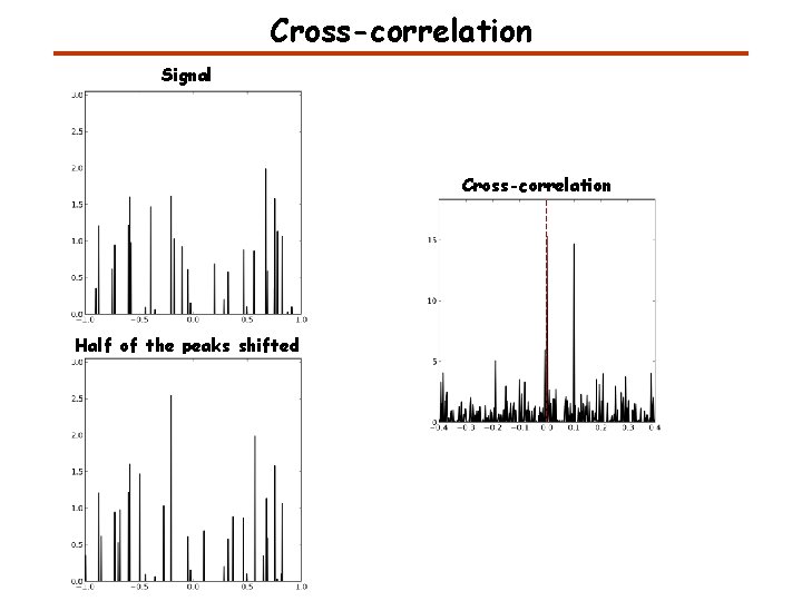
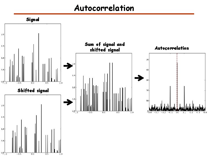
Convolution, Cross-correlation, and Autocorrelation Convolution describes the response of a linear and time-invariant system to an input signal. The inverse Fourier transform of the pointwise product in frequency space. Cross-correlation is a measure of similarity of two signals. Auto-correlation is the cross-correlation of a signal with itself. It can be used for finding a shift between two signals. It can be used for finding periodic signals obscured by noise. http: //en. wikipedia. org/wiki/Convolution

Cross-correlation and autocorrelation http: //en. wikipedia. org/wiki/Convolution

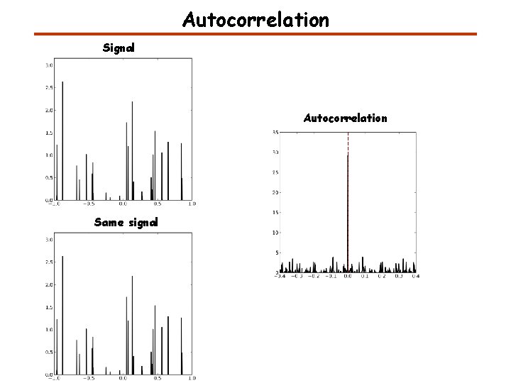
Autocorrelation Signal Autocorrelation Same signal

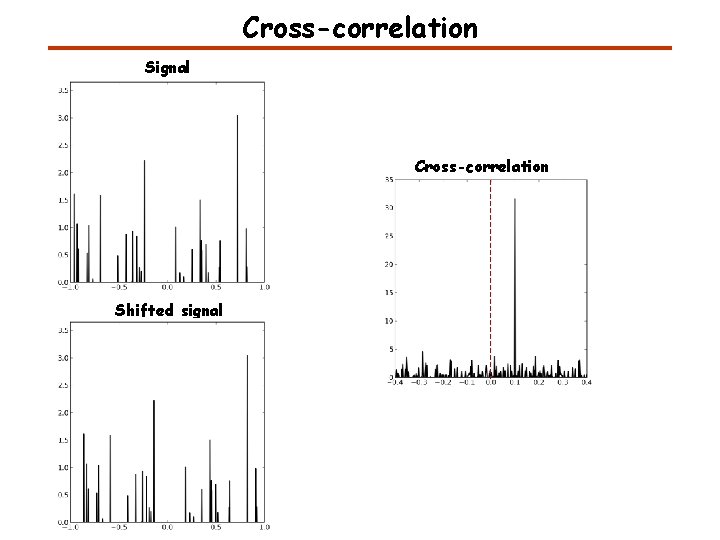
Cross-correlation Signal Cross-correlation Shifted signal

Cross-correlation Signal Cross-correlation Half of the peaks shifted

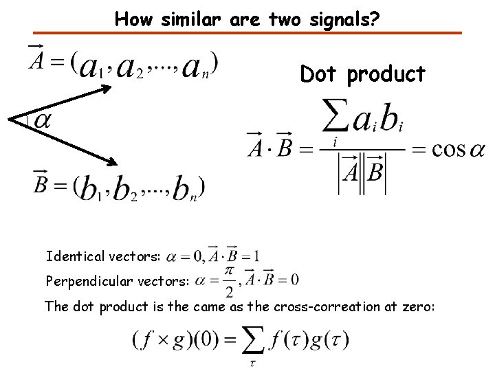
How similar are two signals? Dot product Identical vectors: Perpendicular vectors: The dot product is the came as the cross-correation at zero:

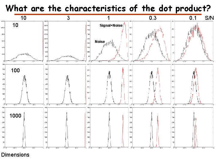
What are the characteristics of the dot product? 10 10 3 1 Signal+Noise 100 1000 Dimensions 0. 3 0. 1 S/N

Autocorrelation Signal Sum of signal and shifted signal Shifted signal Autocorrelation

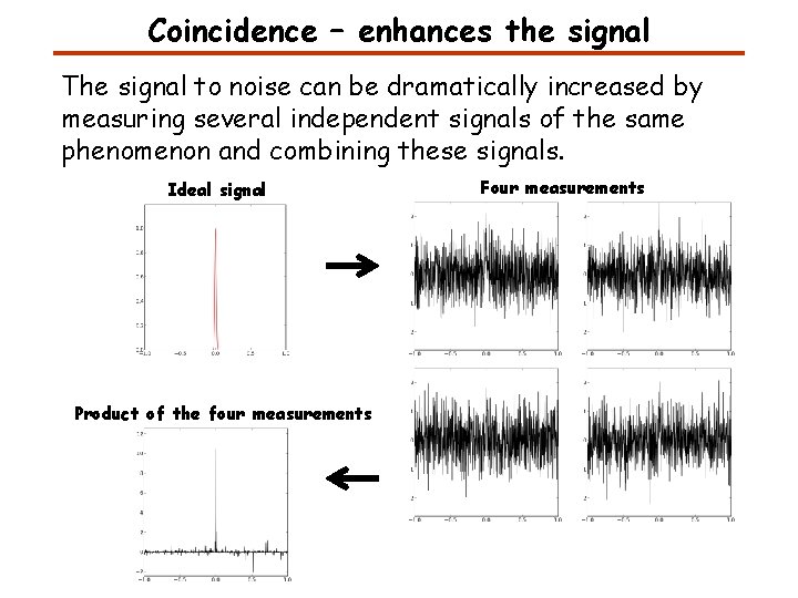
Coincidence – enhances the signal The signal to noise can be dramatically increased by measuring several independent signals of the same phenomenon and combining these signals. Ideal signal Product of the four measurements Four measurements

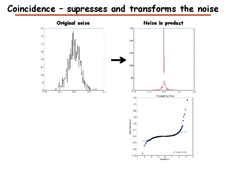
Coincidence – supresses and transforms the noise Original noise Noise in product

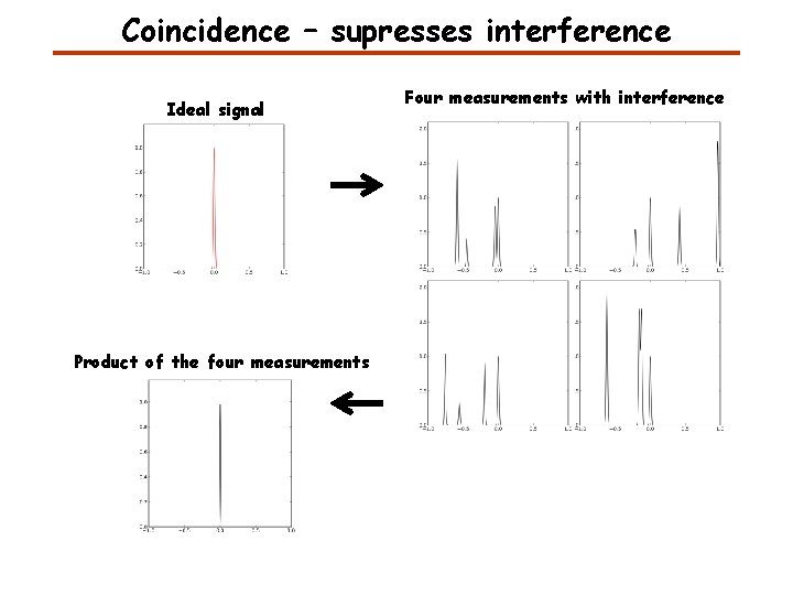
Coincidence – supresses interference Ideal signal Product of the four measurements Four measurements with interference