Sensitivity Analysis Sensitivity analysis refers to the changes

Sensitivity Analysis: Sensitivity analysis refers to the changes in the optimal solution and the optimal value of the objective function due to the changes in the input data coefficients. These changes may occur due to many factors namely price rise, scarcity of raw material, rise or fall in the wages of the labor etc. We will confine ourselves to the following changes in the input data:

A. Changes in the cost coefficients of the objective function. B. Changes in the right hand the side constants. C. Changes in the constraints (Coefficients of Matrix A)

Example: A Dependable company plans production on three products -A, B and C. The unit profits on these products are Rs. 2, Rs. 3 and Rs. 1/ respectively and they require two-resources-labour and raw material. The Company’s O. R. Department formulates the following LPP for determining the optimal product mix.

Max Z=2 x 1+3 x 2+x 3 Sub to x 1, x 2, x 3 ≥ 0 where x 1, x 2, x 3 denote the numbers of the products produced.

Now, we standardize the Max Z=2 x 1+3 x 2+x 3 Sub to x 1, x 2, x 3 ≥ 0

Iteration 0 The initial Simplex table is Cj→ 2 Cb Xb↓ 3 1 y 2 y 3 0 0 y 4 y 5 b 0 x 4 1/3 1/3 1 0 x 5 1 1 7/5 0 1 3 -3 -1 0 0 Z=0 Zj-Cj -2

Iteration 1 Cj→ 2 Cb Xb↓ 3 1 0 0 y 1 y 2 y 3 y 4 y 5 b 0 s 1 1/4 0 -1/4 1/4 3 x 2 1/4 1 7/4 0 3/4 9/4 0 17/4 0 9/4 Z=27/4 Zj-Cj -5/4

The Final Optimal Simplex Table (F) is Cj→ 2 Cb 3 1 0 0 b Xb↓ y 1 y 2 y 3 y 4 y 5 2 x 1 1 0 -1 4 -1 1 3 x 2 0 Zj-Cj 0 1 0 2 3 -1 5 1 1 2 Z=8

A: Case (i): Changes in cost coefficients of a non basic variable of the objective function. In the optimal product mix, product C is not produced because of its low profit of Rs. 1 per unit. We are interested in finding the range on the values of C 3 such that the present solution remains optimal. It is clear that when the profit on C 3 decreases, it has no effect on the present solution.

However, when the increases beyond a certain limit, product C may become profitable to be produced. The table is optimal as long as Z 3 -C 3 ≥ 0. Thus, we take C 3 as a variable i. e. , Z 3 -C 3 =Cby 3 -C 3 ≥ 0 or (2, 3)

-2+6 -C 3≥ 0 or -C 3 ≥-4 or C 3 ≤ 4. Thus, as long as the profit on Product C is up to Rs. 4, it is not economical to produce product C. Suppose, the profit on product C increases to Rs. 6, then Z 3 -C 3=2 and the current product mix is no more optimal

New table with C 3=6 Cj→ 2 Cb 3 6 0 0 b Xb↓ y 1 y 2 y 3 y 4 y 5 2 x 1 1 0 -1 4 -1 1 3 x 2 0 Zj-Cj 0 1 0 2 -2 -1 5 1 1 2 Z=8

The new final table is Cj→ 2 Cb 3 6 0 0 b Xb↓ y 1 y 2 y 3 y 4 y 5 2 x 1 1 1/2 0 7/2 -1/2 1 6 x 3 0 Zj-Cj 0 1/2 1 1 0 -1/2 4 1/2 2 2 Z=10

Thus, the optimal product mix is to produce 2 units of product A and 1 unit of product C with a maximum profit of Rs. 10. Generally, it takes one more iteration to reach the optimal product mix.

Case (ii): Changes in the coefficient of the basic variable • Changing the coefficient of a basic variable: We wish to determine the effect of changes on the unit profit of product A. If the profit on C 1 decreases, then it may not be profitable to produce any more. Even, when the profit increases to a certain level, this product may even become the only product to be produced.

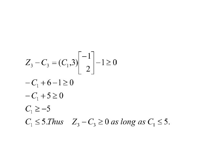
To determine the range on C 1, we observe that change in C 1 changes the profit vector Cb Since Cb=(c 1, c 2), it can be verified that the relative profit coefficients of the basic variables namely Z 3 -C 3, Z 4 -C 4 and Z 5 -C 5 will change. But as long as these Zj-Cj remain nonnegative, the optimal table (F) remains optimal. We express the values of Z 3 -C 3, Z 4 -C 4 and Z 5 -C 5 as a function of C 1

and

also

Thus from the above calculations , C 3 lies between [3/4 , 3]. The table F remains optimal as long as the changes on C 1 are within 3/4 and 3. Of course, the value of the objective function will change. For example when C 1=1, the optimal solution is given by x 1=1, x 2=2 and x 3=0, but the optimal value is 7. When the value of C 1 goes beyond the limit of [3/4, 3], the table F is no more optimal and the Simplex Method has to be applied again.

Case (iii): Changing the price of both basic and non-basic variables: A simple case, we may see the changes in both the variables e. g. , changing the coefficients of basic variables x 1 and x 2 from 2 and 3 to 1 and 4 and of non basic variable x 3 from 1 to 2

The effect on the optimal product table F remains optimal or not.

• Hence the table F remains optimal with x 1=2, x 2=2 and x 3=0 and the optimal value of the objective function is 9. However, it has an indication of an alternative optimal solution.

• B. Change in right hand side constants bi: Let us explore the changes in the optimal product mix if an additional unit of labour is made available. It is clear that this change has no effect on the table F except for changes in the value of the constants. Even after the change, if the right side constants remain nonnegative, then the solution given by table F is still a basic feasible solution and the Zequation of Table F are the same, thus the table F is optimal.

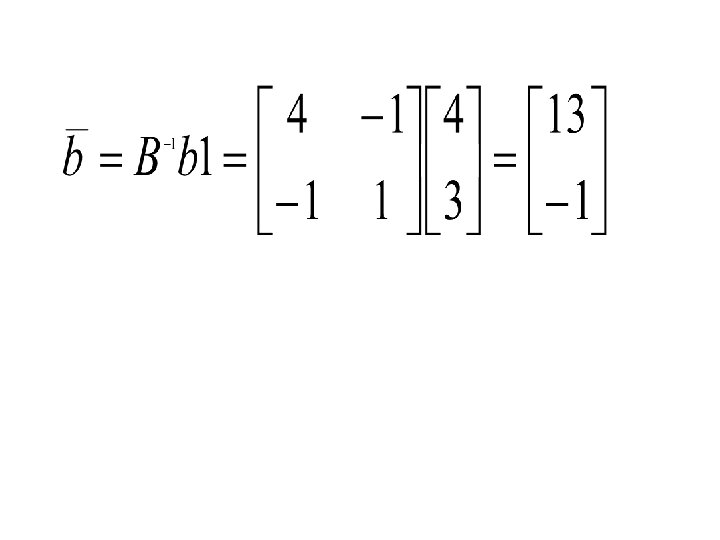
of changes in the right hand side constants (bi), it is sufficient to see whether the new vector of constants in the final table stays non-negative. Thus from Table F, we have,

and the values of new right hand vector with increased labour

which is a positive vector. Hence, Table F is still an optimal table and the new optimal product mix is x 1=5 and x 2=1 and the new optimal value of Z*=13. We note that both the optimal solution and the optimal value have changed due to the changes in the availability of labour but the optimal basis has not changed and the optimal product mix remains unchanged.

Suppose the extra unit of labour is made available by allowing overtime which costs an additional Rs. 4/- to the company. The company may evaluate whether this is economical or not by finding Z 1=Z*-Z=Rs. 13 -Rs. 8=Rs. 5 which is more than the cost of overtime (Rs. 4/-) and it is therefore profitable to get an additional unit of 1 unit of labour. The increased profit of Rs. 5 per unit increase in labour availability is called the shadow price for the labour constraint.

Thus knowing the shadow price of various constraints helps in determining how much one can afford to pay for the increases in the constrained resources. To use the concept of shadow prices, we compute the range on the variation of constraint resources such that the optimal basis remains optimal.

Thus

The optimal solution is x 1=4 b 1 -3, x 2=-b 1+3 and x 3=0. The maximum profit Z=2(4 b 13)+3(-b 1+3) =Rs. 5 b 1+3 Let us consider the case when the labor availability is increased to 4 units. This means

which is not a non-positive vector as required. Thus x 1=13, x 2=-1, x 3=0, x 4=0 and x 5=0 is infeasible.

C: Changes in the Constraint Matrix: The coefficient matrix A may change due to the changes in the following: i) Adding a new variable ii) Changing the resource requirements of the existing activities iii) Adding new constraints

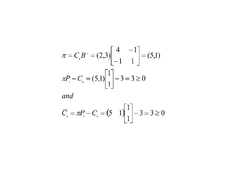
Case i) Suppose, the Cos R & D Department comes out with a proposal to produce which requires 1 unit of labour and 1 unit of material with a unit profit of Rs. 3. The Company would like to know whether it is economical to produce product D or not? .

As we know that inclusion of a new product is equivalent to adding a new variable say x 6 and a column with in initial table (Iteration 0) table 1. Thus table 1 is optimal as long Z 6 -C 6 is nonnegative. We use Revised Simplex Method,

Since no variable qualifies to enter into the basis, the Table F remains optimal. This means that producing product D will not improve the solution i. e. , the profit can not be improved. Similarly, the two other cases in (ii) and (iii) will be dealt with.