2 3 Sensitivity Analysis Sensitivity analysis is defined

2. 3. Sensitivity Analysis § Sensitivity analysis is defined as a study of how the uncertainty in the output of a mathematical model can be apportioned, qualitatively or quantitatively, to different sources of variation in the input of a model. § A main purpose of sensitivity analysis is to identify the sensitive parameters. 1

Cont… § When linear programming was formulated, it was implicitly assumed that the parameters of the model were known with certainty. § However, rarely does a manager know all of these parameters exactly. § In reality the model parameters are simply estimates that are subject to change. § For this reason it is of interest to the manager to see what effects a change in a parameter will have on the solution to the model. 2

Cont… § Change may be either reactions to anticipated uncertainties in the parameters or reactions to information. § The analysis of parameter changes and their effects on the model solution is known as sensitivity. 3

Cont… § To ascertain the effect of a change in the parameter of a model is: I. to make the change in the original model II. resolve the model and III. compare the solution results with original. 4

Cont… § Some parameters of change: I. Objective function coefficient II. Constraints quantity value ( RHS) III. Coefficient of the constraints IV. Deletion of constraints V. Addition of constraints VI. Addition and deletion of variables etc 5

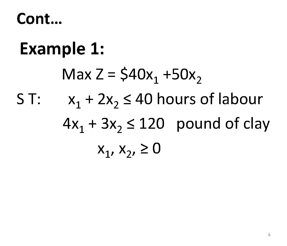
Cont… Example 1: S T: Max Z = $40 x 1 +50 x 2 x 1 + 2 x 2 ≤ 40 hours of labour 4 x 1 + 3 x 2 ≤ 120 pound of clay x 1, x 2, ≥ 0 6

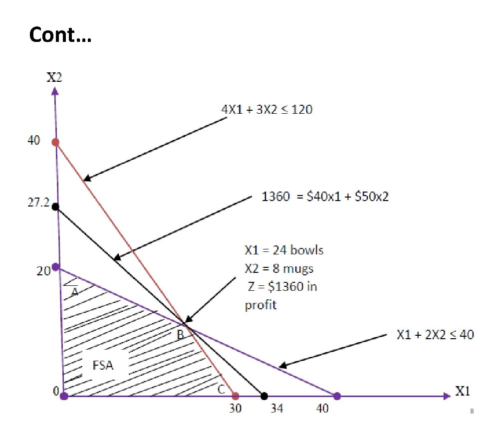
Cont… I. Objective Function Coefficient Ranges § The first model parameter change we will analyse is a change in an objective function coefficient. We will use the above given model to illustrate this change. § Graphical solution for this problem is shown below 7

Cont… 8

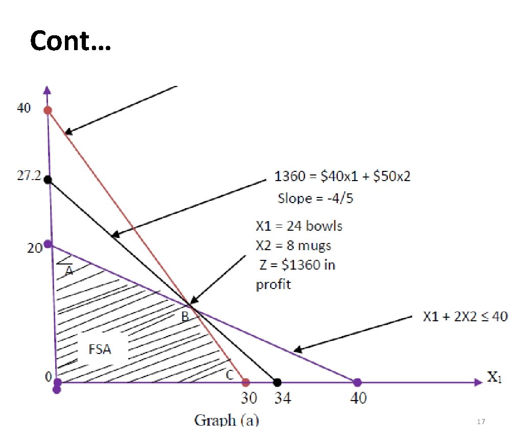
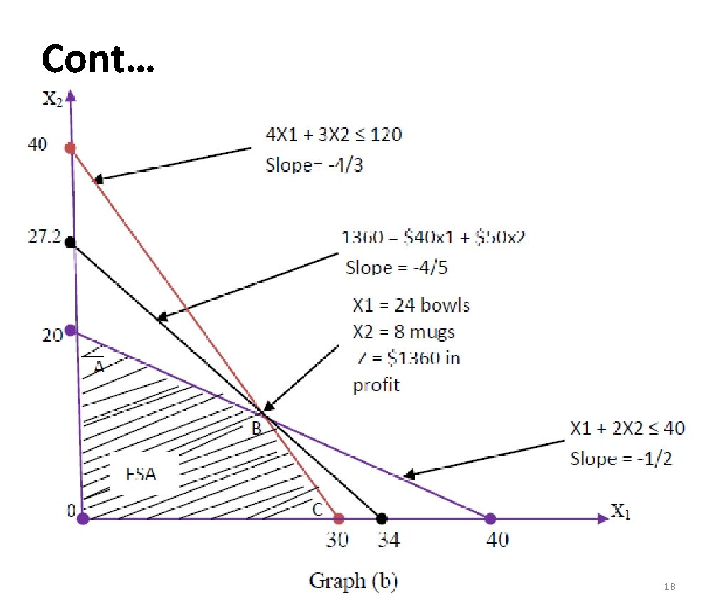
Cont… § The optimal solution point is shown to be at corner point B (x 1 = 24, x 2 =8), which is the last point the objective function line touches as it leaves the feasible solution area. § However, what will happen if we change the profit of a bowl, x 1, from $40 to $100? How would that affect the solution identified previous? 9

Cont… 10

Cont… § Increasing profit for a bowl , i. e. , the x 1 coefficient , from $40 to $100 made the objective function line steeper , so much so that the optimal solution point changed from corner point B to corner point C. § If we had increased the profit for a mug , the x 2 coefficient , from $50 to $100 , the objective function line would have become flatter to the extent that corner point A would become optimal with x 1=0, x 2 = 20 and Z = $2000. 11

Cont… § The objective of sensitivity analysis in this case is to determine the range of values for a specific objective function coefficient over which the optimal solution point, x 1 and x 2, will remain optimal. 12

Cont… § E. g. the coefficient of x 1 in the objective function is originally $40, but at some value greater than $40, point C will become optimal, and at some value less than $40, point A will become optimal. The focus of sensitivity analysis is to determine those two values, referred to as the sensitivity range for x 1 coefficient, which we will designate as C 1. 13

Cont… § Look at the graph above and determine the sensitivity range for x 1 coefficient. The slope of the objective function is currently -4/5, determined as follows. § Z = 40 x 1 +50 x 2, So, X 2 = Z/50 – 4 x 1/5 § The objective function is now in the form of the equation of a straight line, Y =a+Bx, where the intercept, a, equal 1/50 and the slope, b, is -4/5. 14

Cont… § If the slope of the objective function increases into -4/3, the objective function line becomes exactly parallel to the constraint line. 4 x 1 + 3 x 2 = 120 And point C becomes optimal (along with B). The slope of this constraint line is -4/3, so we ask ourselves what objective function coefficient for x 1 will make the objective function slope equal -4/3. The answer is determined as follows, where C 1 is the objective function coefficient for x 1, 15

Cont… § -C 1/50 = -4/3, § -3 C 1=-200 , C 1 = $66. 67, § X 2 Slope = -4/3 16

Cont… 17

Cont… 18

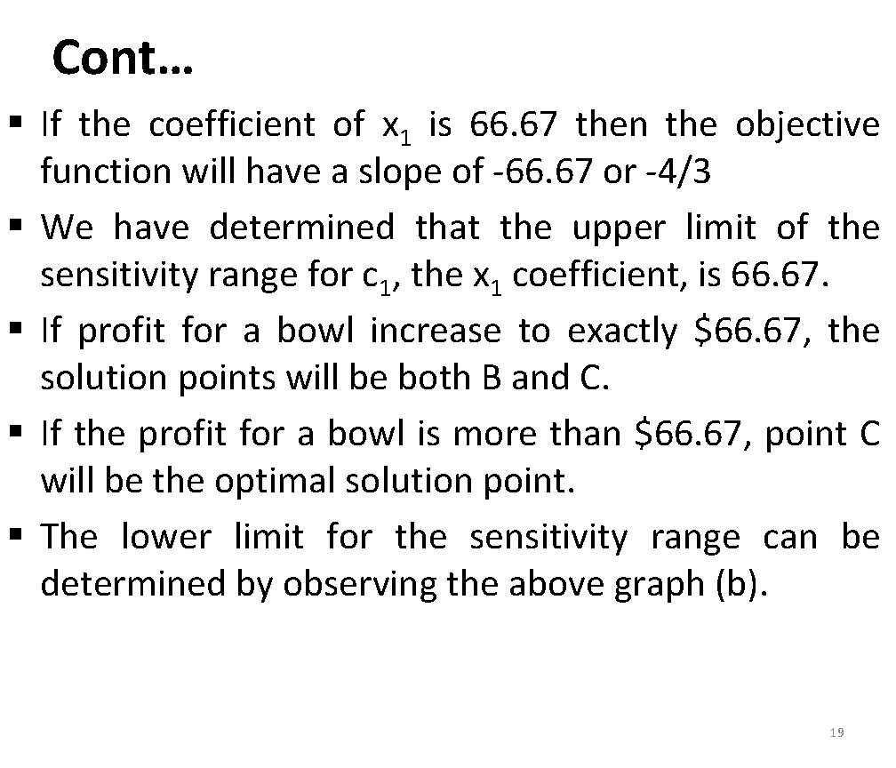
Cont… § If the coefficient of x 1 is 66. 67 then the objective function will have a slope of -66. 67 or -4/3 § We have determined that the upper limit of the sensitivity range for c 1, the x 1 coefficient, is 66. 67. § If profit for a bowl increase to exactly $66. 67, the solution points will be both B and C. § If the profit for a bowl is more than $66. 67, point C will be the optimal solution point. § The lower limit for the sensitivity range can be determined by observing the above graph (b). 19

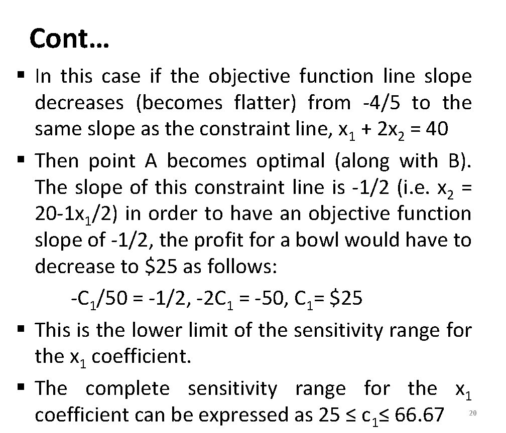
Cont… § In this case if the objective function line slope decreases (becomes flatter) from -4/5 to the same slope as the constraint line, x 1 + 2 x 2 = 40 § Then point A becomes optimal (along with B). The slope of this constraint line is -1/2 (i. e. x 2 = 20 -1 x 1/2) in order to have an objective function slope of -1/2, the profit for a bowl would have to decrease to $25 as follows: -C 1/50 = -1/2, -2 C 1 = -50, C 1= $25 § This is the lower limit of the sensitivity range for the x 1 coefficient. § The complete sensitivity range for the x 1 coefficient can be expressed as 25 ≤ c 1≤ 66. 67 20

Cont… § This means that the profit for a bowl can vary anywhere between $25 and $66. 67 and the optimal solution point, x 1 = 24 and X 2 = 8, will not change. Of course, the total profit, or Z value, will change depending on whatever value c 1 actually is. 21

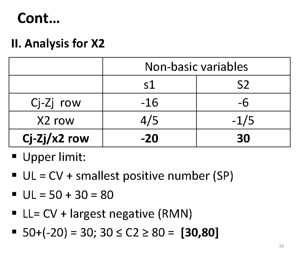
Cont… § Performing the same type of graphical analysis will provide the sensitivity range for the x 2 objective function coefficient, c 2. This range is 30 ≤ c 2 ≤ 80. This means that the profit for a mug can vary between $30 and $80 and the optimal solution Point, B, will not change. § when we say that profit for a mug can vary between $30 and $80; this is true only if C 1 remains constant. 22

Cont… § Simultaneous changes can be made in the objective coefficients as long as change taken together does not exceed 100% of the total allowable changes for all the ranges combined § E. g. The maximum allowable increase in the profit for a bowl, according to the upper limit of the sensitivity range, $66. 67 $40 = $26. 67. the maximum allowable increase for a mug is $80 -$50 = $30. 23

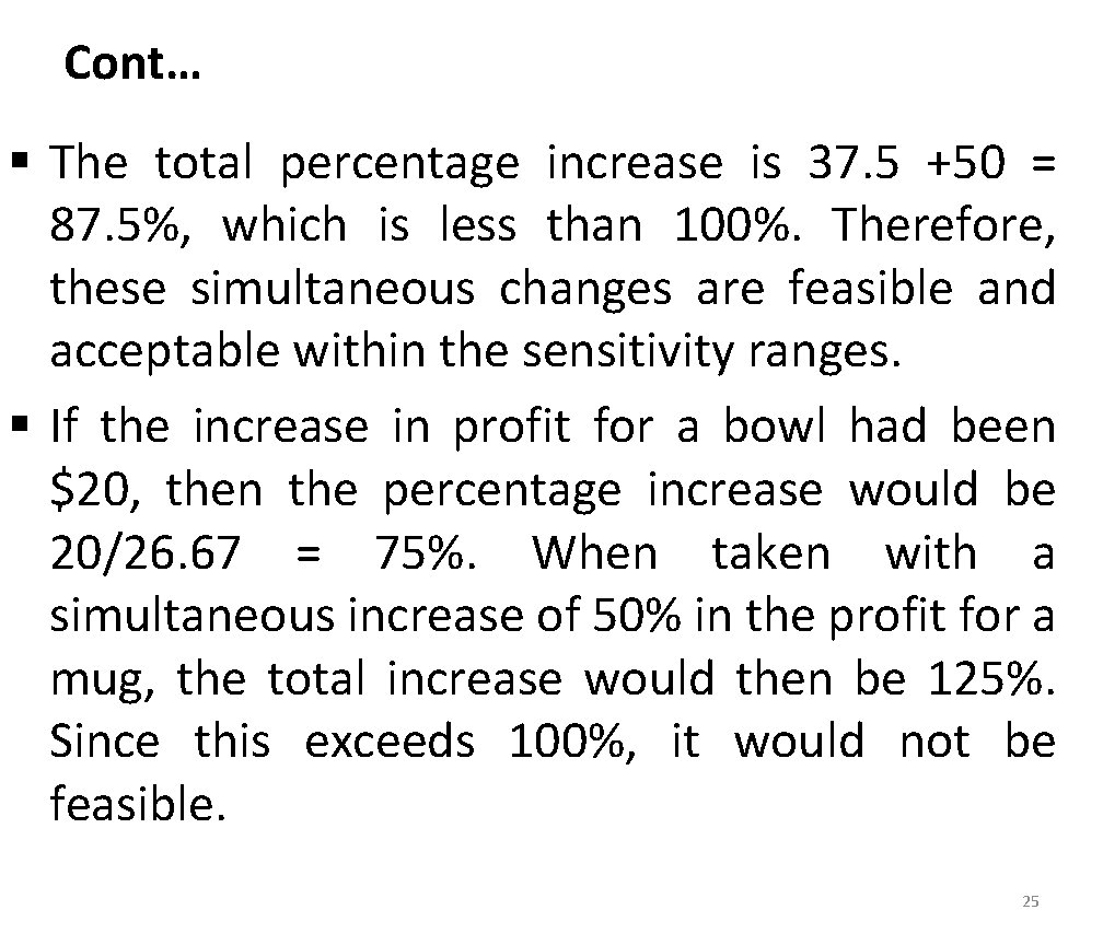
Cont… § What if the profit for a bowl is increased by $10 and the profit for a mug is increased by $15? Ten dollar is $10/26. 67 x 100 = 37. 5% of the maximum allowable increases for a bowl’s profit, and $15 is 15/30 = 50% of the maximum allowable increase in the profit for a mug. 24

Cont… § The total percentage increase is 37. 5 +50 = 87. 5%, which is less than 100%. Therefore, these simultaneous changes are feasible and acceptable within the sensitivity ranges. § If the increase in profit for a bowl had been $20, then the percentage increase would be 20/26. 67 = 75%. When taken with a simultaneous increase of 50% in the profit for a mug, the total increase would then be 125%. Since this exceeds 100%, it would not be feasible. 25

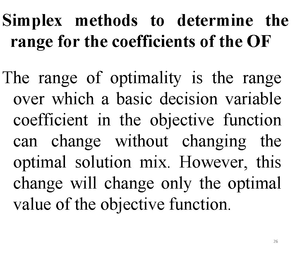
Simplex methods to determine the range for the coefficients of the OF The range of optimality is the range over which a basic decision variable coefficient in the objective function can change without changing the optimal solution mix. However, this change will change only the optimal value of the objective function. 26

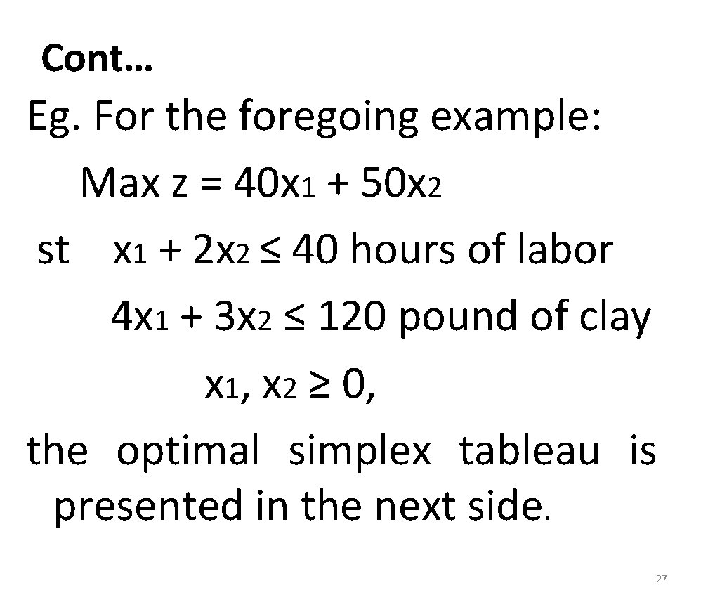
Cont… Eg. For the foregoing example: Max z = 40 x 1 + 50 x 2 st x 1 + 2 x 2 ≤ 40 hours of labor 4 x 1 + 3 x 2 ≤ 120 pound of clay x 1, x 2 ≥ 0, the optimal simplex tableau is presented in the next side. 27

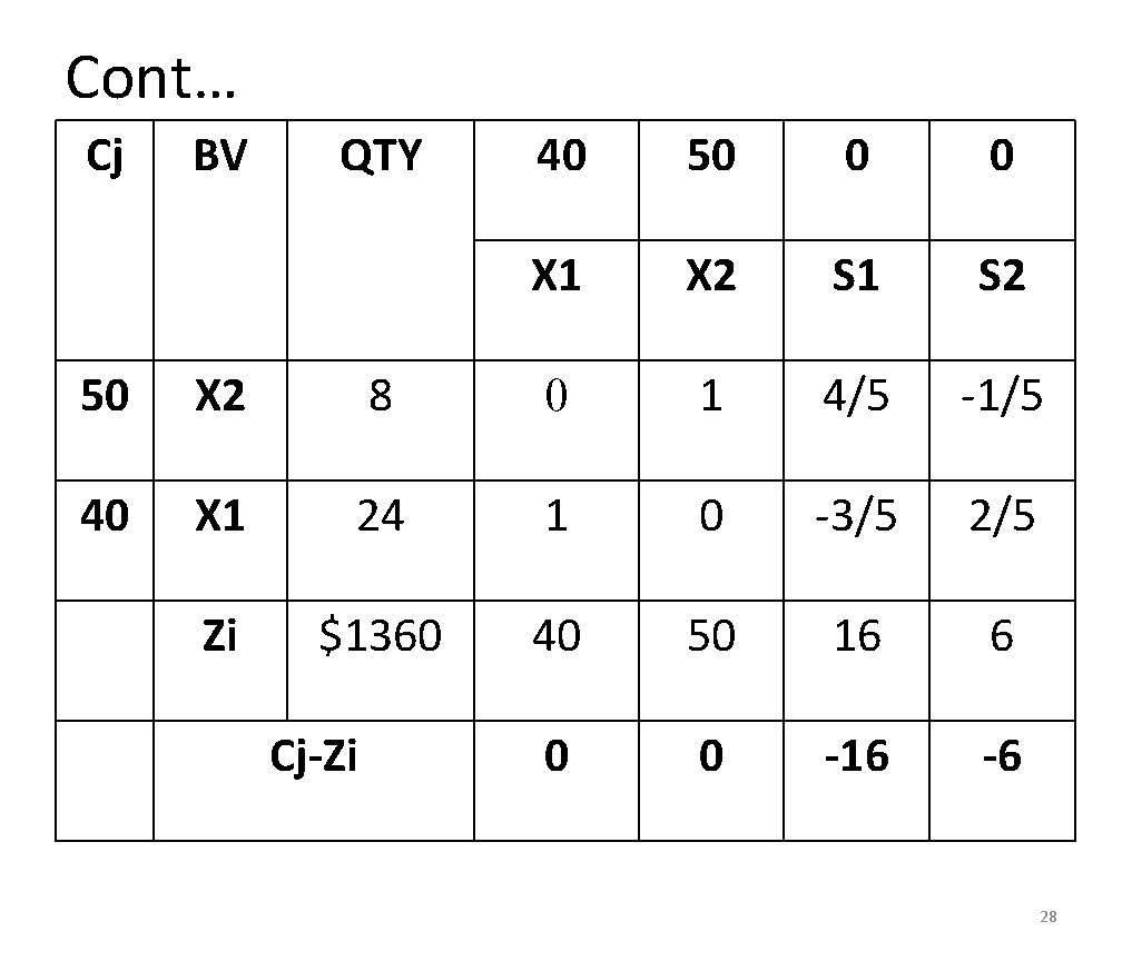
Cont… Cj BV QTY 40 50 0 0 X 1 X 2 S 1 S 2 50 X 2 8 0 1 4/5 -1/5 40 X 1 24 1 0 -3/5 2/5 Zi $1360 40 50 16 6 0 0 -16 -6 Cj-Zi 28

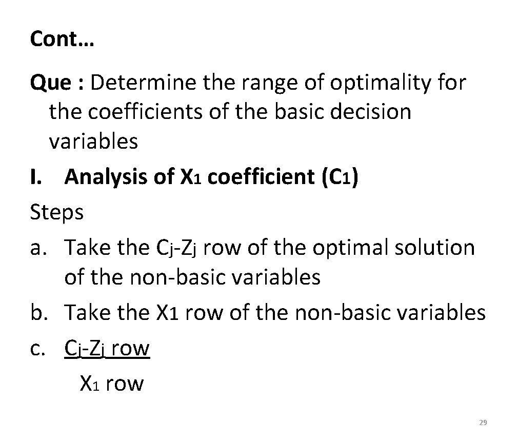
Cont… Que : Determine the range of optimality for the coefficients of the basic decision variables I. Analysis of X 1 coefficient (C 1) Steps a. Take the Cj-Zj row of the optimal solution of the non-basic variables b. Take the X 1 row of the non-basic variables c. Cj-Zj row X 1 row 29

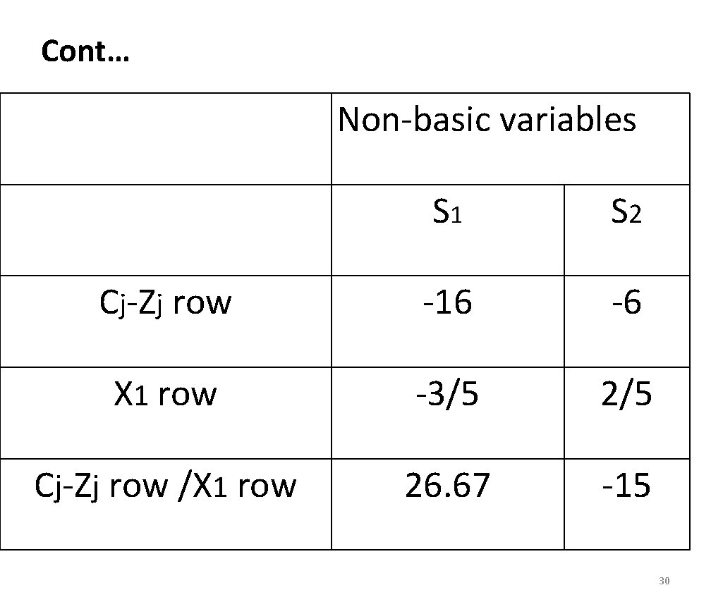
Cont… Non-basic variables S 1 S 2 Cj-Zj row -16 -6 X 1 row -3/5 2/5 Cj-Zj row /X 1 row 26. 67 -15 30

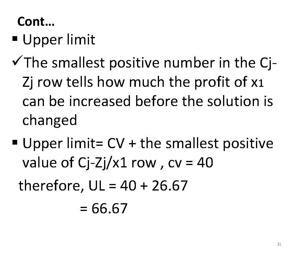
Cont… § Upper limit üThe smallest positive number in the Cj. Zj row tells how much the profit of x 1 can be increased before the solution is changed § Upper limit= CV + the smallest positive value of Cj-Zj/x 1 row , cv = 40 therefore, UL = 40 + 26. 67 = 66. 67 31

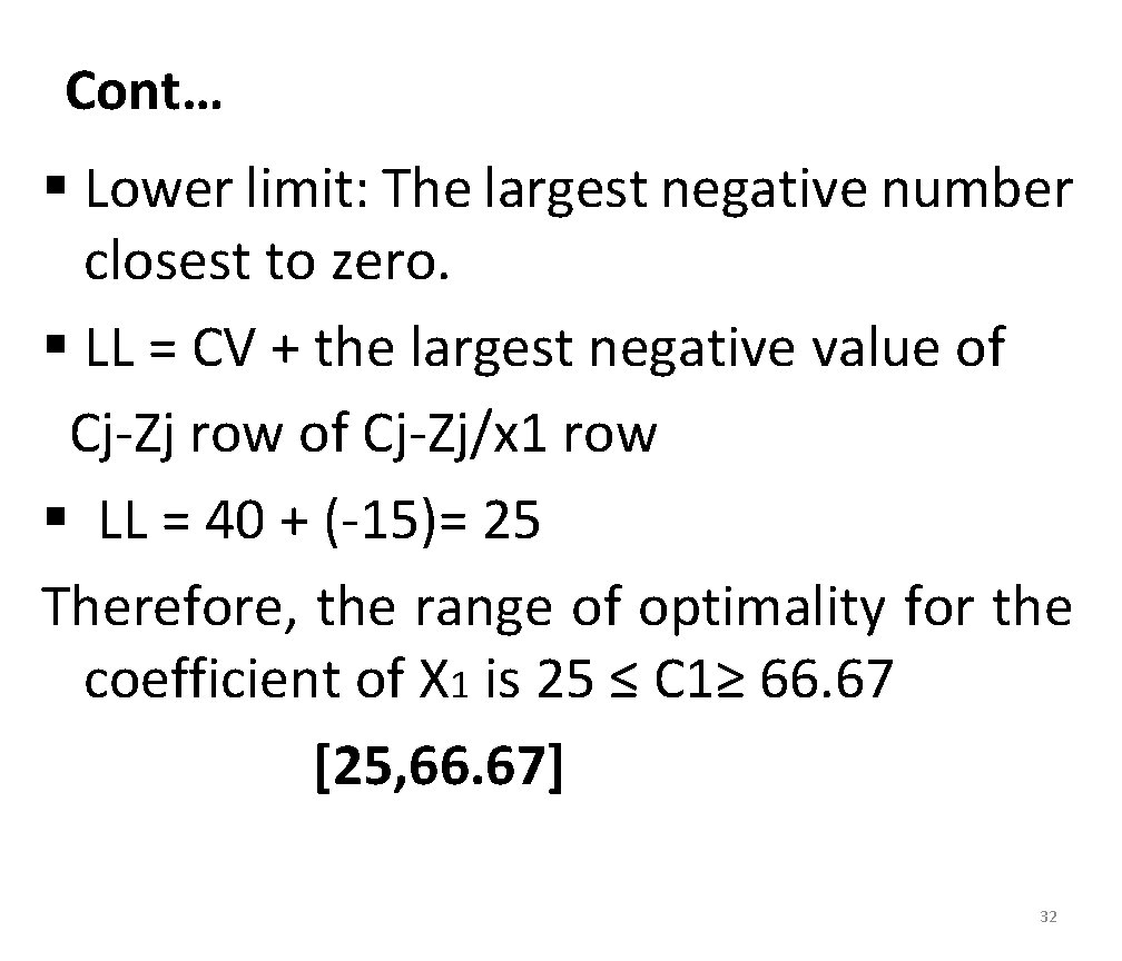
Cont… § Lower limit: The largest negative number closest to zero. § LL = CV + the largest negative value of Cj-Zj row of Cj-Zj/x 1 row § LL = 40 + (-15)= 25 Therefore, the range of optimality for the coefficient of X 1 is 25 ≤ C 1≥ 66. 67 [25, 66. 67] 32

Cont… II. Analysis for X 2 Non-basic variables s 1 S 2 -16 -6 4/5 -1/5 -20 30 § § § Cj-Zj row X 2 row Cj-Zj/x 2 row Upper limit: UL = CV + smallest positive number (SP) UL = 50 + 30 = 80 LL= CV + largest negative (RMN) 50+(-20) = 30; 30 ≤ C 2 ≥ 80 = [30, 80] 33

II. Changes in Constraint Quantity Values (RHS) Using graphical solution method Shadow prices: how much should a firm be willing to pay to make additional resources available? Shadow price signify the changes in the optimal value of the objective function for 1 unit increases in the value of the RHS of the constraint that represent the availability of scarce resources. The negative number of Cj –Zj row is its slack variable columns provide as with shadow prices RHS ranging is the range over which shadow prices remain valid 34

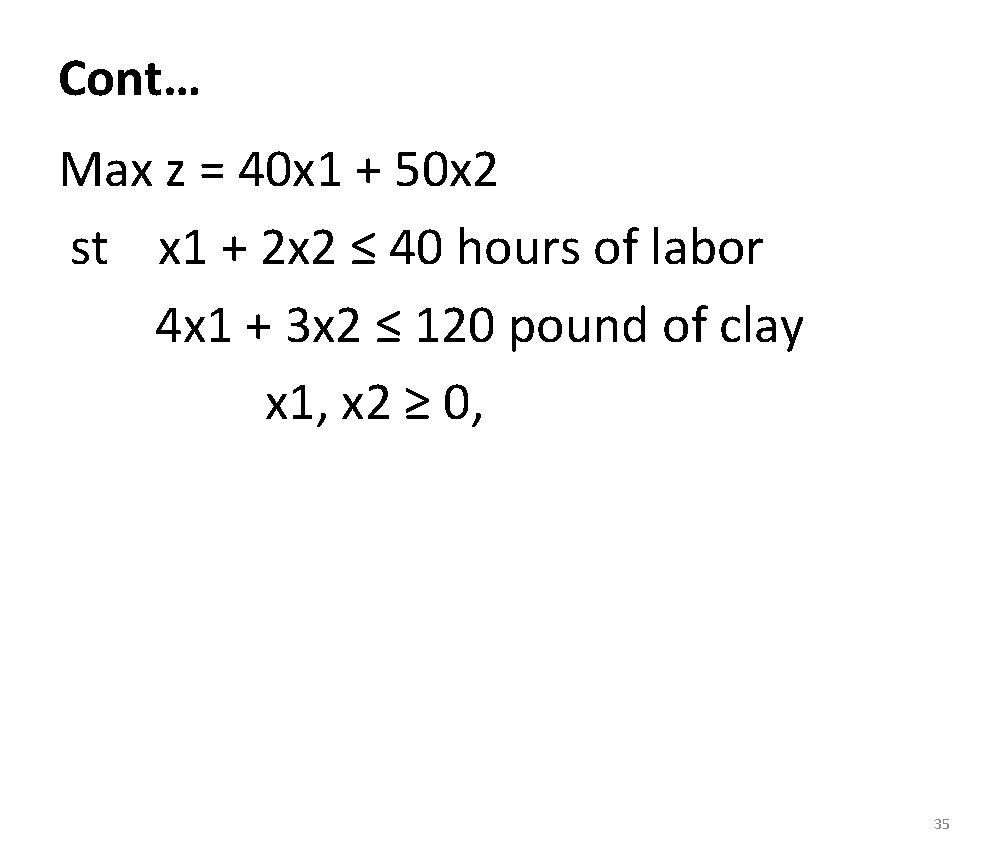
Cont… Max z = 40 x 1 + 50 x 2 st x 1 + 2 x 2 ≤ 40 hours of labor 4 x 1 + 3 x 2 ≤ 120 pound of clay x 1, x 2 ≥ 0, 35

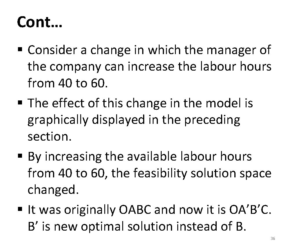
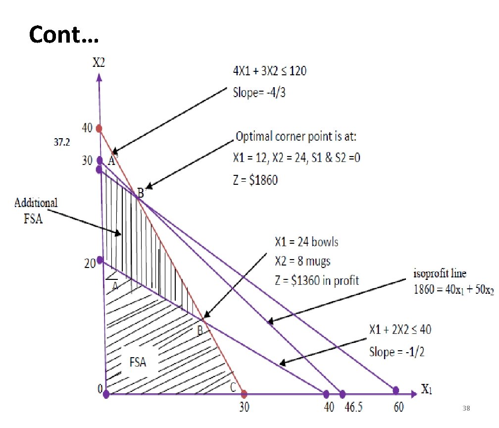
Cont… § Consider a change in which the manager of the company can increase the labour hours from 40 to 60. § The effect of this change in the model is graphically displayed in the preceding section. § By increasing the available labour hours from 40 to 60, the feasibility solution space changed. § It was originally OABC and now it is OA’B’C. B’ is new optimal solution instead of B. 36

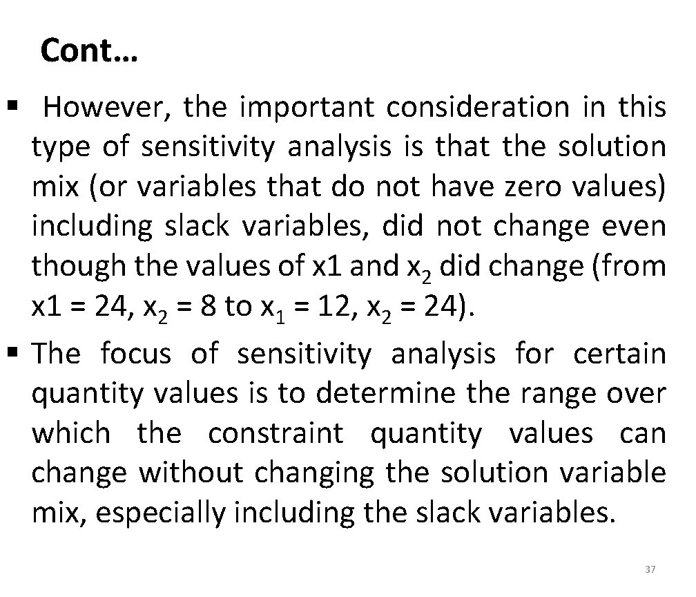
Cont… § However, the important consideration in this type of sensitivity analysis is that the solution mix (or variables that do not have zero values) including slack variables, did not change even though the values of x 1 and x 2 did change (from x 1 = 24, x 2 = 8 to x 1 = 12, x 2 = 24). § The focus of sensitivity analysis for certain quantity values is to determine the range over which the constraint quantity values can change without changing the solution variable mix, especially including the slack variables. 37

Cont… 38

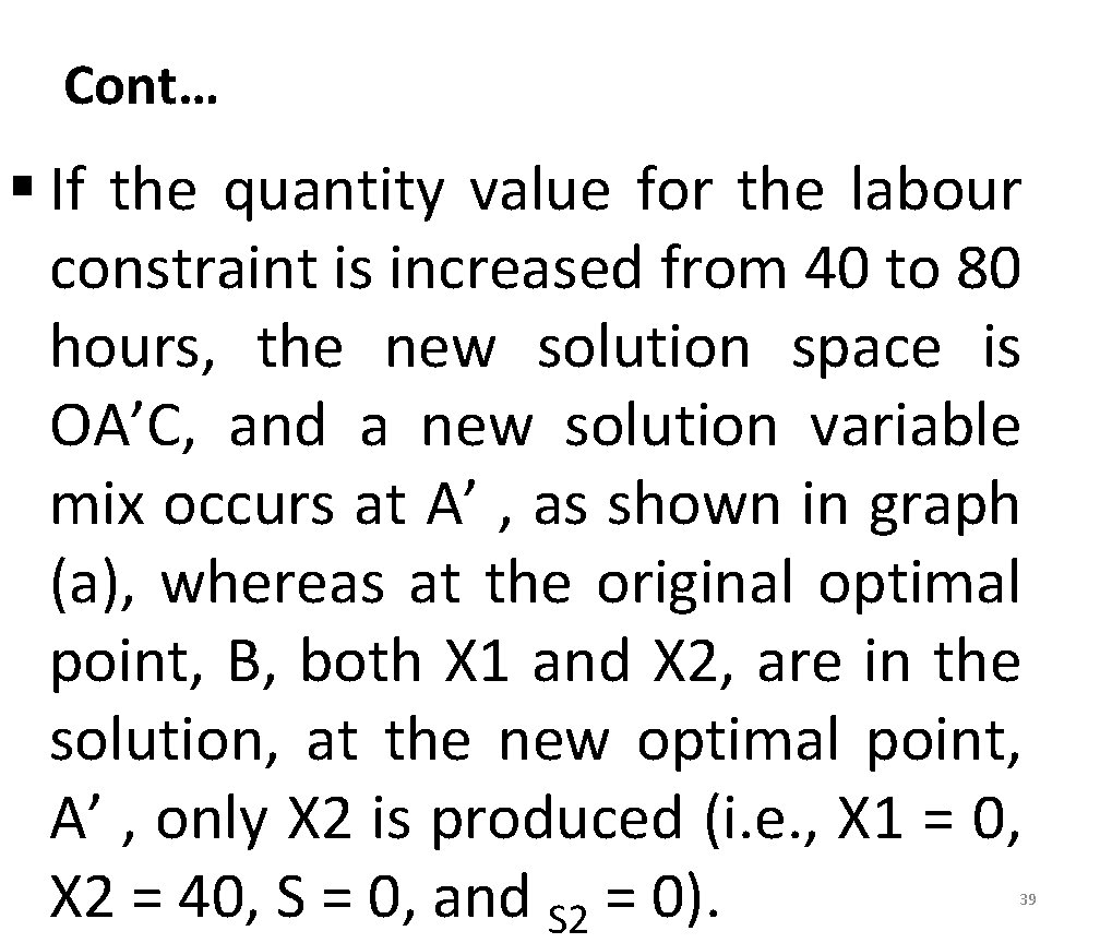
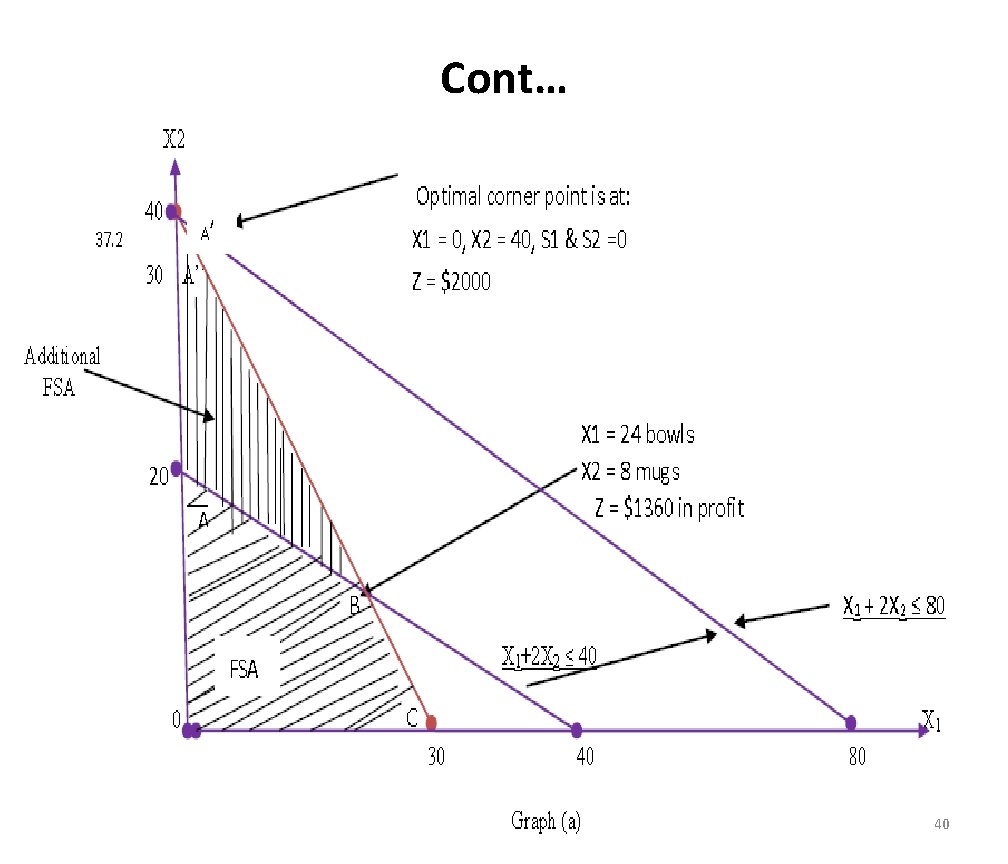
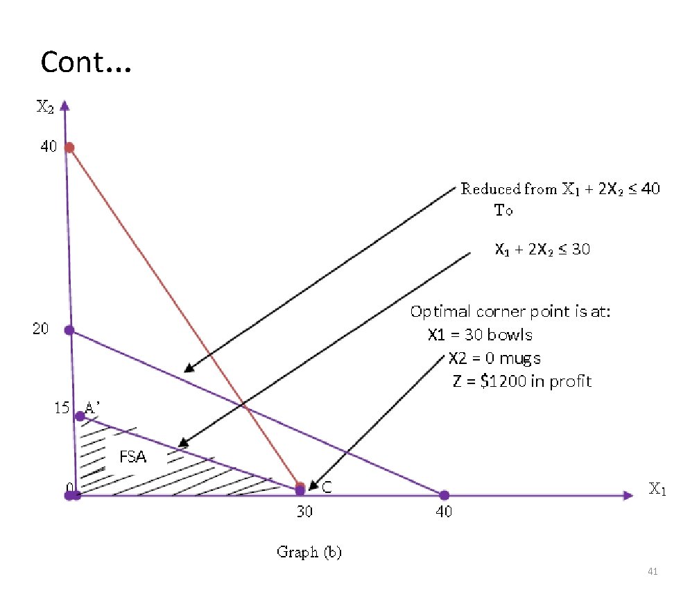
Cont… § If the quantity value for the labour constraint is increased from 40 to 80 hours, the new solution space is OA’C, and a new solution variable mix occurs at A’ , as shown in graph (a), whereas at the original optimal point, B, both X 1 and X 2, are in the solution, at the new optimal point, A’ , only X 2 is produced (i. e. , X 1 = 0, X 2 = 40, S = 0, and S 2 = 0). 39

Cont… 40

Cont… 41

Cont… § The upper limit of the sensitivity range for the quantity value of the first constraint, which we will refer to as q 1 is 8 hours. At this value the solution mix changes such that bowls are no longer produced. Further, as q 1 increases past 80 hours, s 1 increases, i. e. , slack hours are created. Similarly, if the value for q 1 is decreased to 30 hours, the new feasible solution space 42

Cont… is OA’C, as shown in graph (b) above. The new optimal is at C, where no mugs (x 2) are produced. The new solution is x 1 = 30, x 2 = 0, S 1 = 0, S 2 = 0, and Z = $1200. Again, the variable mix is changed. Summarising, the sensitivity range for the constraint quantity value for labour hours is 30 ≤ q 1≤ 80 hours 43

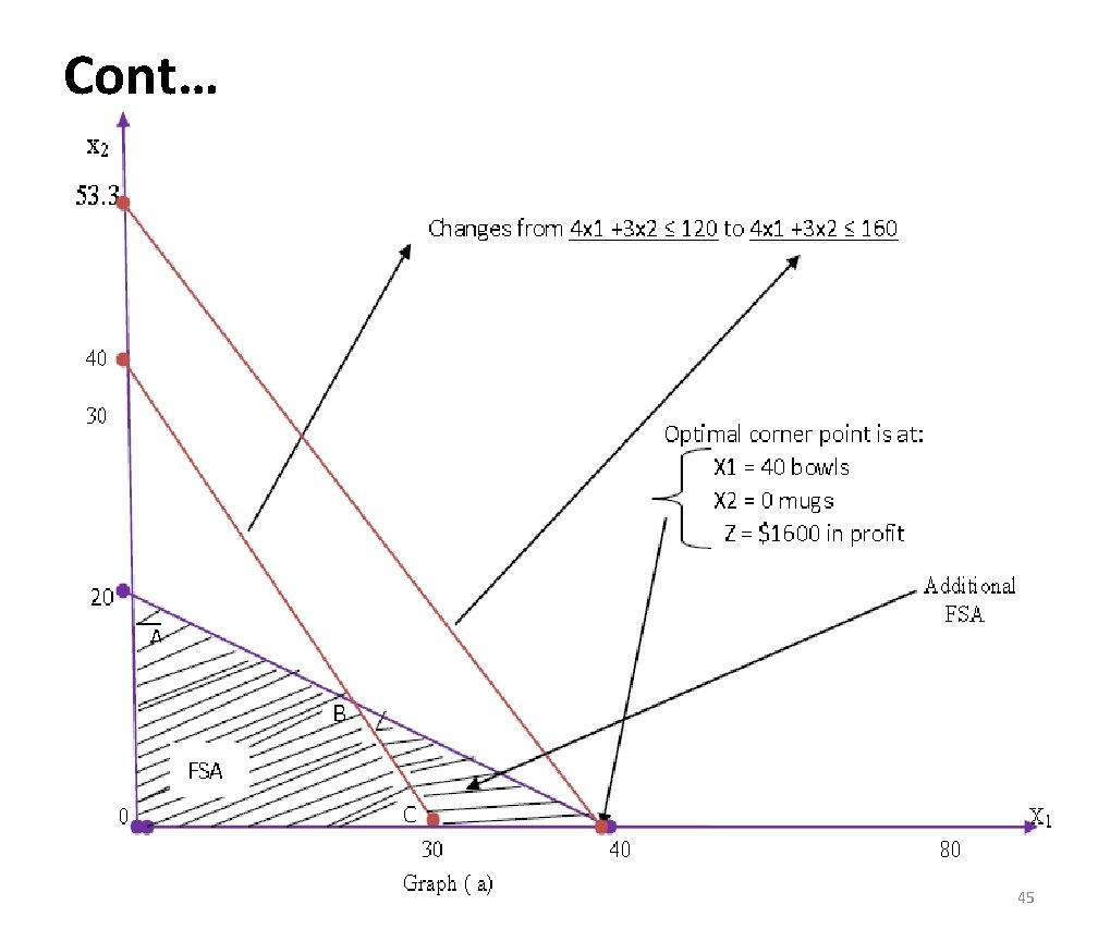
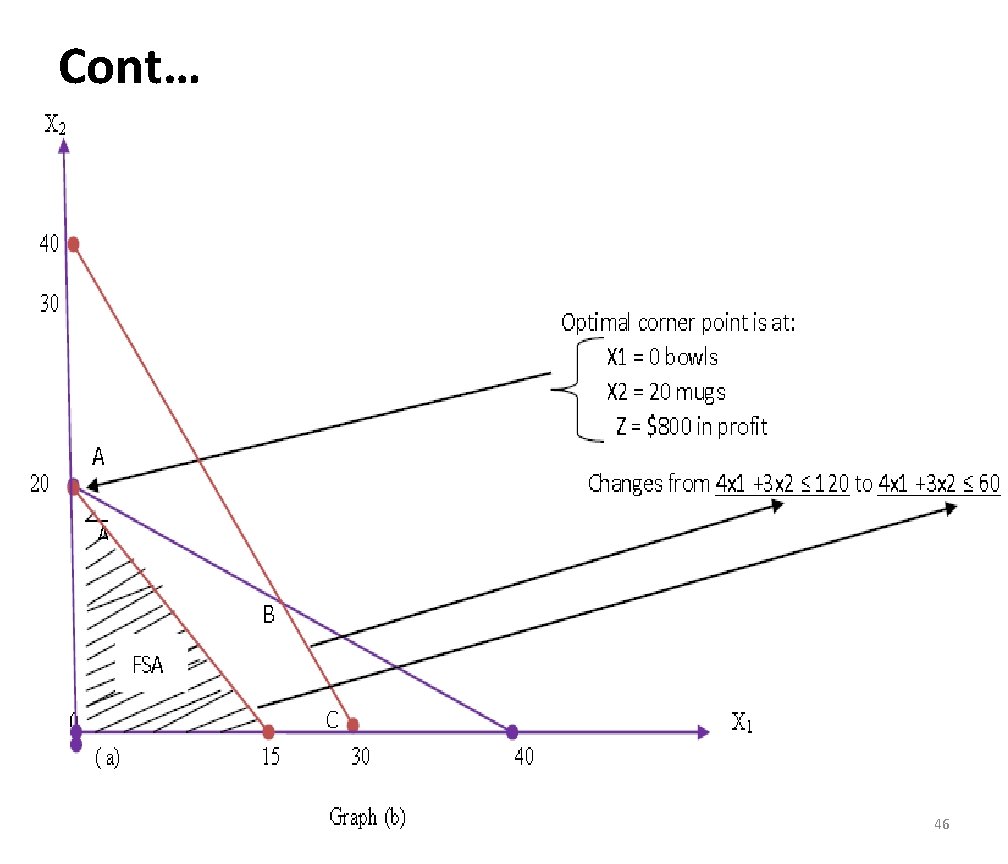
Cont… § The sensitivity range for clay can be determined graphically in a similar manner. If the quantity value for the clay constraint, 4 x 1 + 3 x 2 ≤ 120, is increased from 120 to 160, shown in graph (a) below, then the new solution space , OAC’ , results , with a new optimal point, C’. Alternatively, if the quantity value is decreased from 120 to 60, as shown in graph (b) below, the new solution space is OAC’ and the new optimal point A ( x 1, 20, x 2 =0, S 1=0, S 2= 0, Z= 800) 44

Cont… 45

Cont… 46

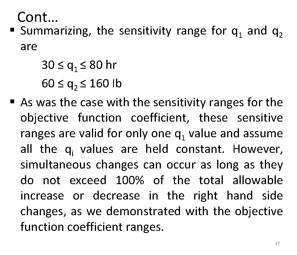
Cont… § Summarizing, the sensitivity range for q 1 and q 2 are 30 ≤ q 1 ≤ 80 hr 60 ≤ q 2 ≤ 160 Ib § As was the case with the sensitivity ranges for the objective function coefficient, these sensitive ranges are valid for only one q 1 value and assume all the qi values are held constant. However, simultaneous changes can occur as long as they do not exceed 100% of the total allowable increase or decrease in the right hand side changes, as we demonstrated with the objective function coefficient ranges. 47

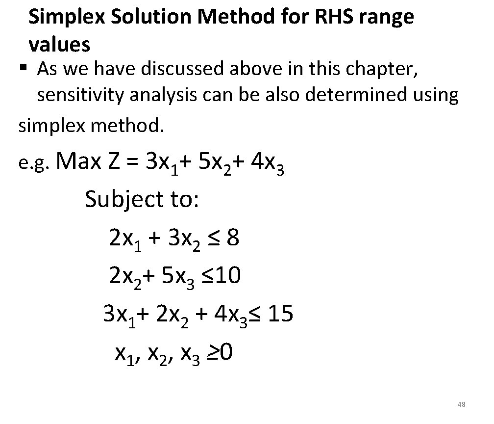
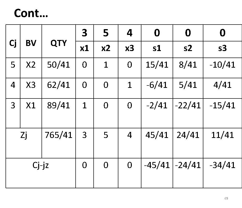
Simplex Solution Method for RHS range values § As we have discussed above in this chapter, sensitivity analysis can be also determined using simplex method. e. g. Max Z = 3 x 1+ 5 x 2+ 4 x 3 Subject to: 2 x 1 + 3 x 2 ≤ 8 2 x 2+ 5 x 3 ≤ 10 3 x 1+ 2 x 2 + 4 x 3≤ 15 x 1, x 2, x 3 ≥ 0 48

Cont… Cj BV QTY 3 5 4 0 0 0 x 1 x 2 x 3 s 1 s 2 s 3 5 X 2 50/41 0 15/41 8/41 -10/41 4 X 3 62/41 0 0 1 -6/41 5/41 4/41 3 X 1 89/41 1 0 0 -2/41 -22/41 -15/41 765/41 3 5 4 45/41 24/41 0 0 -45/41 -24/41 -34/41 Zj Cj-jz 0 11/41 49

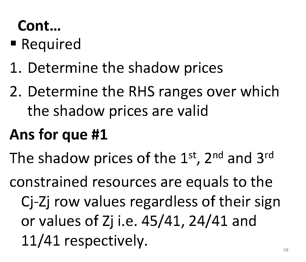
Cont… § Required 1. Determine the shadow prices 2. Determine the RHS ranges over which the shadow prices are valid Ans for que #1 st nd rd The shadow prices of the 1 , 2 and 3 constrained resources are equals to the Cj-Zj row values regardless of their sign or values of Zj i. e. 45/41, 24/41 and 11/41 respectively. 50

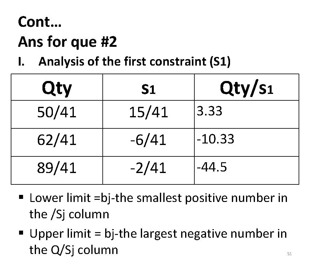
Cont… Ans for que #2 I. Analysis of the first constraint (S 1) Qty s 1 Qty/s 1 50/41 15/41 3. 33 62/41 -6/41 -10. 33 89/41 -2/41 -44. 5 § Lower limit =bj-the smallest positive number in the /Sj column § Upper limit = bj-the largest negative number in the Q/Sj column 51

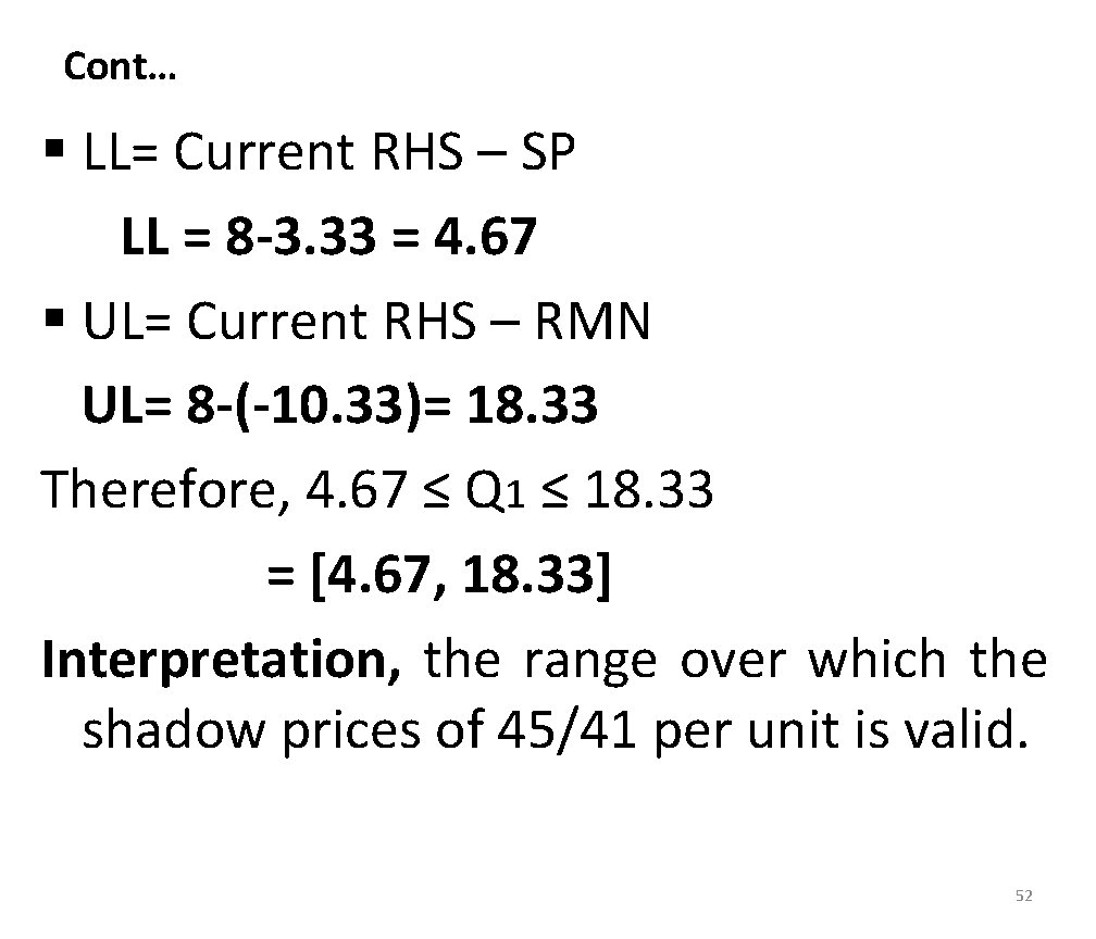
Cont… § LL= Current RHS – SP LL = 8 -3. 33 = 4. 67 § UL= Current RHS – RMN UL= 8 -(-10. 33)= 18. 33 Therefore, 4. 67 ≤ Q 1 ≤ 18. 33 = [4. 67, 18. 33] Interpretation, the range over which the shadow prices of 45/41 per unit is valid. 52

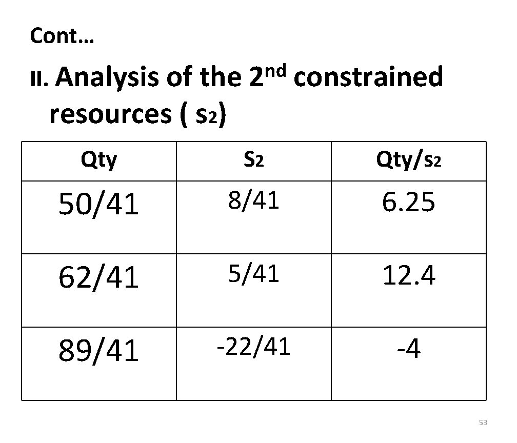
Cont… II. Analysis of the resources ( s 2) nd 2 constrained Qty S 2 Qty/s 2 50/41 8/41 6. 25 62/41 5/41 12. 4 89/41 -22/41 -4 53

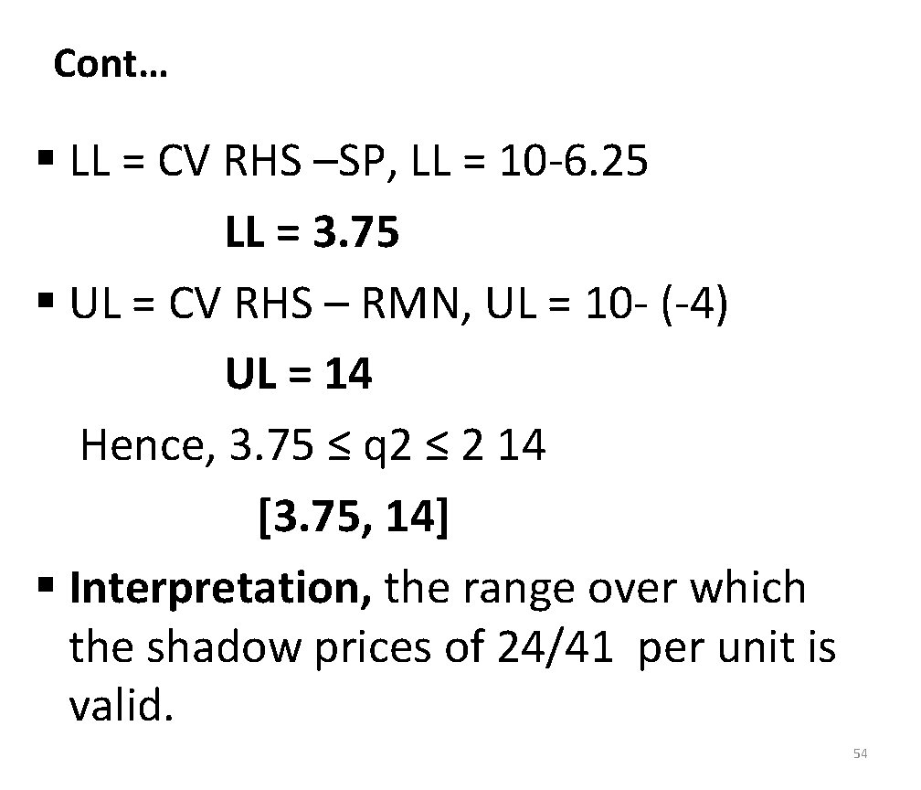
Cont… § LL = CV RHS –SP, LL = 10 -6. 25 LL = 3. 75 § UL = CV RHS – RMN, UL = 10 - (-4) UL = 14 Hence, 3. 75 ≤ q 2 ≤ 2 14 [3. 75, 14] § Interpretation, the range over which the shadow prices of 24/41 per unit is valid. 54

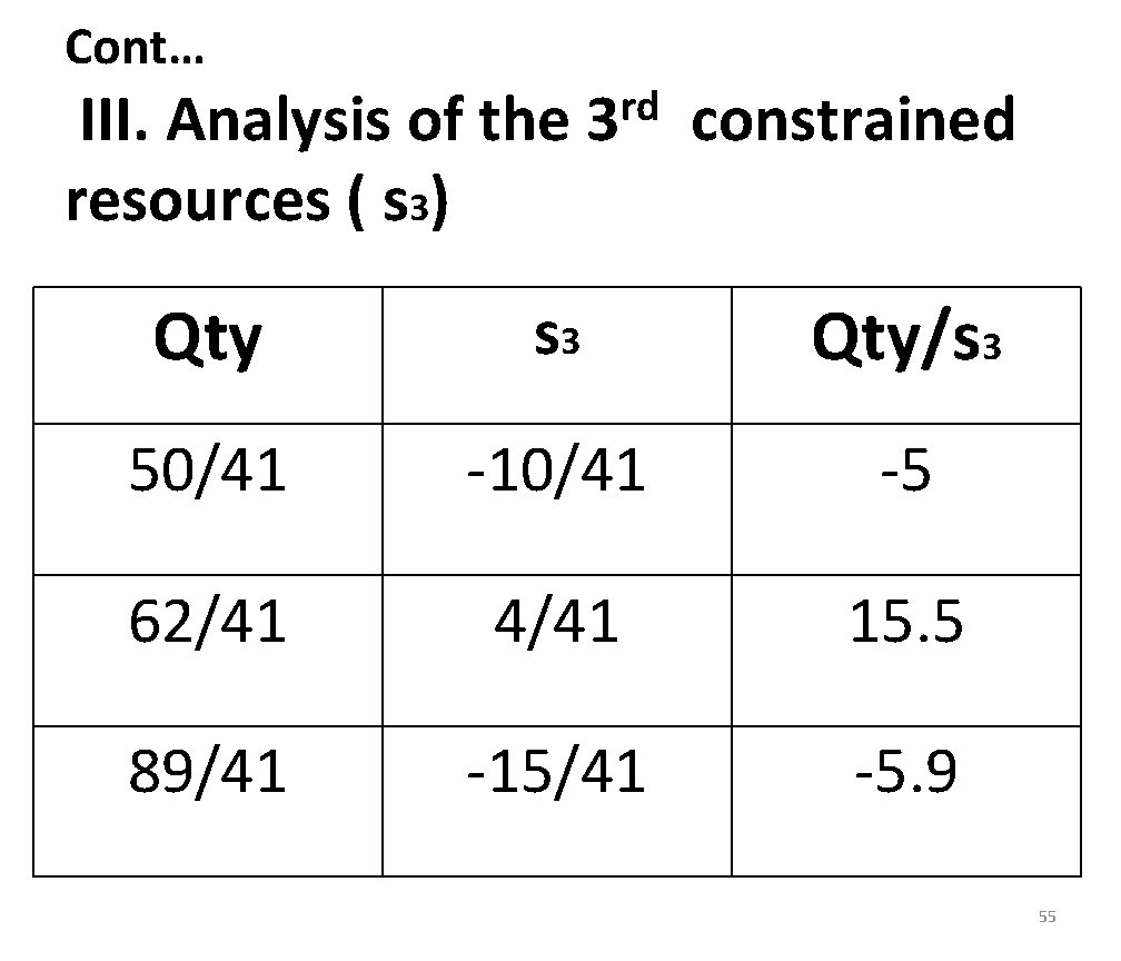
Cont… III. Analysis of the resources ( s 3) rd 3 constrained Qty s 3 Qty/s 3 50/41 -10/41 -5 62/41 4/41 15. 5 89/41 -15/41 -5. 9 55

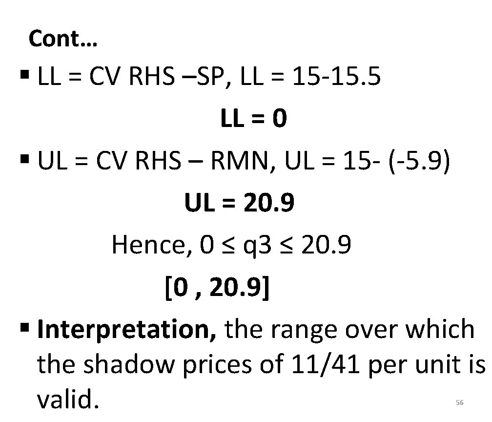
Cont… § LL = CV RHS –SP, LL = 15 -15. 5 LL = 0 § UL = CV RHS – RMN, UL = 15 - (-5. 9) UL = 20. 9 Hence, 0 ≤ q 3 ≤ 20. 9 [0 , 20. 9] § Interpretation, the range over which the shadow prices of 11/41 per unit is valid. 56

Characteristics of OFC and RHS Change v. Characteristics of Objective Function Coefficient Changes § There is no effect on the feasible region § The slope of the level profit line changes § If the slope changes enough, a different corner point will become optimal § There is a range for each OFC where the current optimal corner point remains optimal. § If the OFC changes beyond that range a new corner point becomes optimal. 57

Cont… v. Characteristics of RHS Changes § The constraint line shifts, which could change the feasible region § Slope of constraint line does not change § Corner point locations can change § The optimal solution can change 58