Section 7 2 Estimating a Population Proportion Copyright

Section 7 -2 Estimating a Population Proportion Copyright © 2010, 2007, 2004 Pearson Education, Inc. 7. 1 - 1

Definition The sample proportion is the best point estimate of the population proportion. sample proportion where x is the number of occurrences observed in the sample size n Copyright © 2010, 2007, 2004 Pearson Education, Inc. 7. 1 - 2

Example: In the Chapter Problem we noted that in a Pew Research Center poll, 1051 of 1501 randomly selected adults in the United States believe in global warming, so the sample proportion is = 0. 70. Find the best point estimate of the proportion of all adults in the United States who believe in global warming. Because the sample proportion is the best point estimate of the population proportion, we conclude that the best point estimate of p is 0. 70. When using the sample results to estimate the percentage of all adults in the United States who believe in global warming, the best estimate is 70%. Copyright © 2010, 2007, 2004 Pearson Education, Inc. 7. 1 - 3

Definition A confidence interval (or interval estimate) is a range (or an interval) of values used to estimate the true value of a population parameter. A confidence interval is sometimes abbreviated as CI. Copyright © 2010, 2007, 2004 Pearson Education, Inc. 7. 1 - 4

Definition A confidence level is the probability 1 – α (often expressed as the equivalent percentage value) that the confidence interval actually does contain the population parameter, assuming that the estimation process is repeated a large number of times. (The value α is later called significance level. ) Most common choices are 90%, 95%, or 99%. (α = 10%), (α = 5%), (α = 1%) Copyright © 2010, 2007, 2004 Pearson Education, Inc. 7. 1 - 5

Interpreting a Confidence Interval We must be careful to interpret confidence intervals correctly. There is a correct interpretation and many different and creative incorrect interpretations of the confidence interval 0. 677 < p < 0. 723. “We are 95% confident that the interval from 0. 677 to 0. 723 actually does contain the true value of the population proportion p. ” This means that if we were to select many different samples of size 1501 and construct the corresponding confidence intervals, 95% of them would actually contain the value of the population proportion p. (Note that in this correct interpretation, the level of 95% refers to the success rate of the process being used to estimate the proportion. ) Copyright © 2010, 2007, 2004 Pearson Education, Inc. 7. 1 - 6

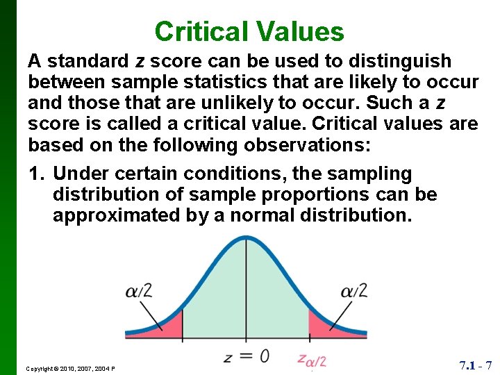
Critical Values A standard z score can be used to distinguish between sample statistics that are likely to occur and those that are unlikely to occur. Such a z score is called a critical value. Critical values are based on the following observations: 1. Under certain conditions, the sampling distribution of sample proportions can be approximated by a normal distribution. Copyright © 2010, 2007, 2004 Pearson Education, Inc. 7. 1 - 7

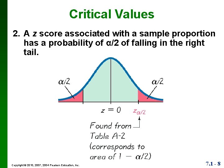
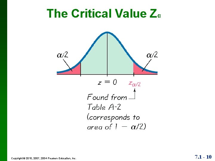
Critical Values 2. A z score associated with a sample proportion has a probability of α/2 of falling in the right tail. Copyright © 2010, 2007, 2004 Pearson Education, Inc. 7. 1 - 8

Critical Values 3. The z score separating the right-tail region is commonly denoted by Zα and is referred to as a critical value because it is on the borderline separating z scores from sample proportions that are likely to occur from those that are unlikely to occur. Copyright © 2010, 2007, 2004 Pearson Education, Inc. 7. 1 - 9

The Critical Value Zα Copyright © 2010, 2007, 2004 Pearson Education, Inc. 7. 1 - 10

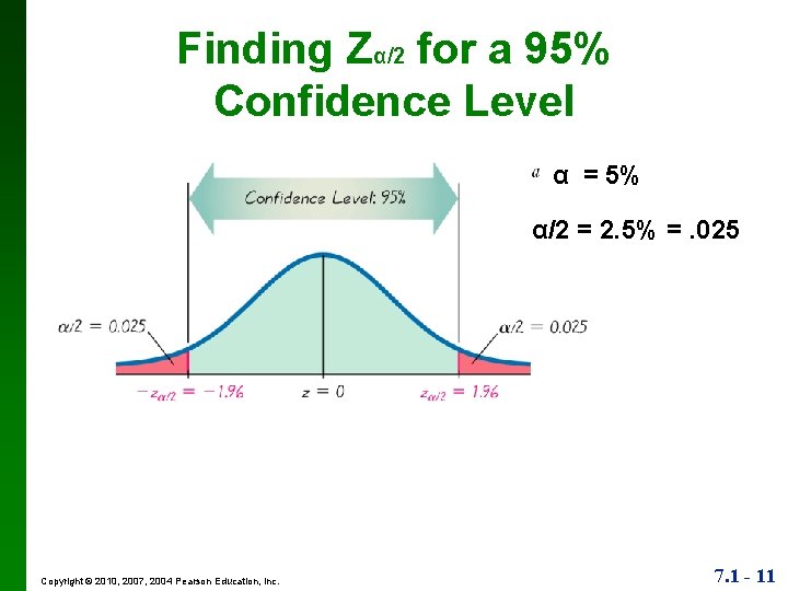
Finding Zα/2 for a 95% Confidence Level α = 5% α/2 = 2. 5% =. 025 Copyright © 2010, 2007, 2004 Pearson Education, Inc. 7. 1 - 11

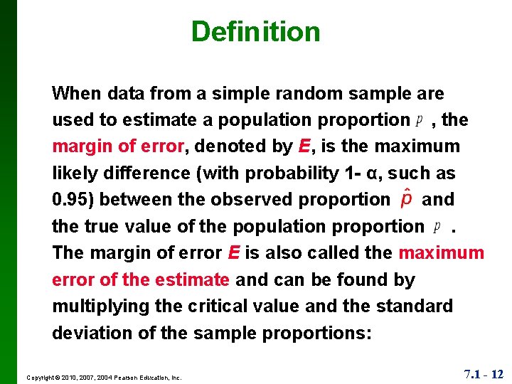
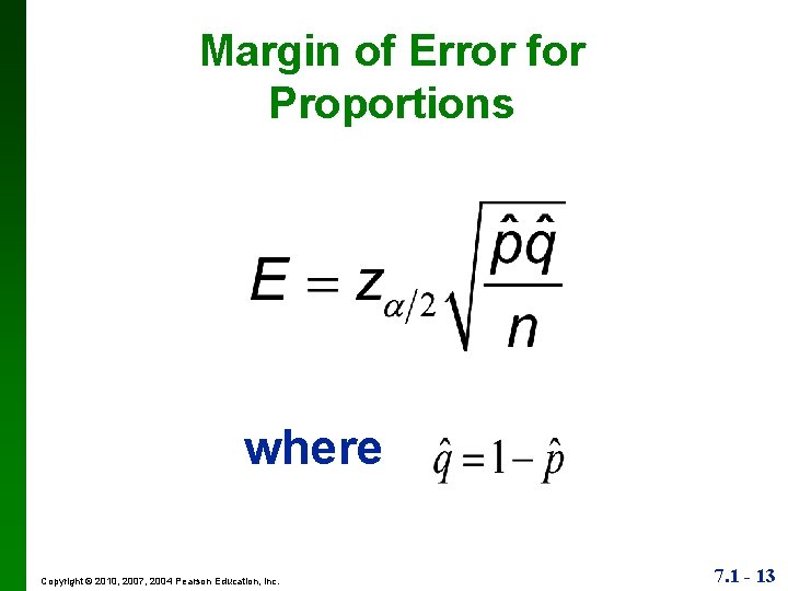
Definition When data from a simple random sample are used to estimate a population proportion , the margin of error, denoted by E, is the maximum likely difference (with probability 1 - α, such as 0. 95) between the observed proportion and the true value of the population proportion. The margin of error E is also called the maximum error of the estimate and can be found by multiplying the critical value and the standard deviation of the sample proportions: Copyright © 2010, 2007, 2004 Pearson Education, Inc. 7. 1 - 12

Margin of Error for Proportions where Copyright © 2010, 2007, 2004 Pearson Education, Inc. 7. 1 - 13

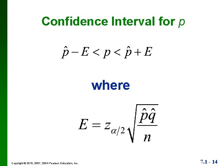
Confidence Interval for p where Copyright © 2010, 2007, 2004 Pearson Education, Inc. 7. 1 - 14

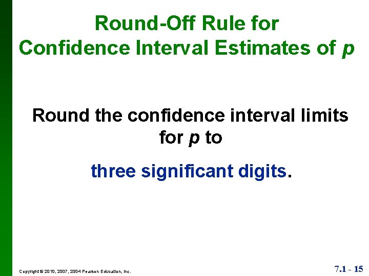
Round-Off Rule for Confidence Interval Estimates of p Round the confidence interval limits for p to three significant digits. Copyright © 2010, 2007, 2004 Pearson Education, Inc. 7. 1 - 15

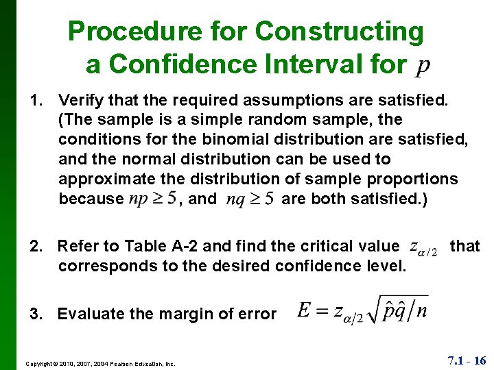
Procedure for Constructing a Confidence Interval for 1. Verify that the required assumptions are satisfied. (The sample is a simple random sample, the conditions for the binomial distribution are satisfied, and the normal distribution can be used to approximate the distribution of sample proportions because , and are both satisfied. ) 2. Refer to Table A-2 and find the critical value corresponds to the desired confidence level. that 3. Evaluate the margin of error Copyright © 2010, 2007, 2004 Pearson Education, Inc. 7. 1 - 16

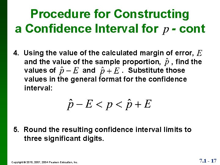
Procedure for Constructing a Confidence Interval for - cont 4. Using the value of the calculated margin of error, and the value of the sample proportion, , find the values of and. Substitute those values in the general format for the confidence interval: 5. Round the resulting confidence interval limits to three significant digits. Copyright © 2010, 2007, 2004 Pearson Education, Inc. 7. 1 - 17

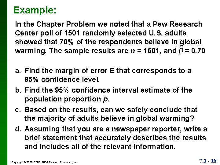
Example: In the Chapter Problem we noted that a Pew Research Center poll of 1501 randomly selected U. S. adults showed that 70% of the respondents believe in global warming. The sample results are n = 1501, and = 0. 70 a. Find the margin of error E that corresponds to a 95% confidence level. b. Find the 95% confidence interval estimate of the population proportion p. c. Based on the results, can we safely conclude that the majority of adults believe in global warming? d. Assuming that you are a newspaper reporter, write a brief statement that accurately describes the results and includes all of the relevant information. Copyright © 2010, 2007, 2004 Pearson Education, Inc. 7. 1 - 18

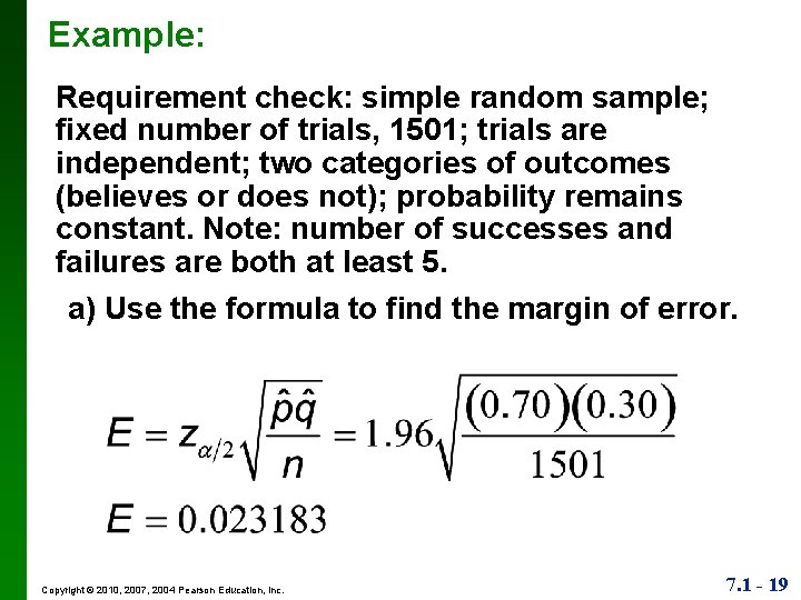
Example: Requirement check: simple random sample; fixed number of trials, 1501; trials are independent; two categories of outcomes (believes or does not); probability remains constant. Note: number of successes and failures are both at least 5. a) Use the formula to find the margin of error. Copyright © 2010, 2007, 2004 Pearson Education, Inc. 7. 1 - 19

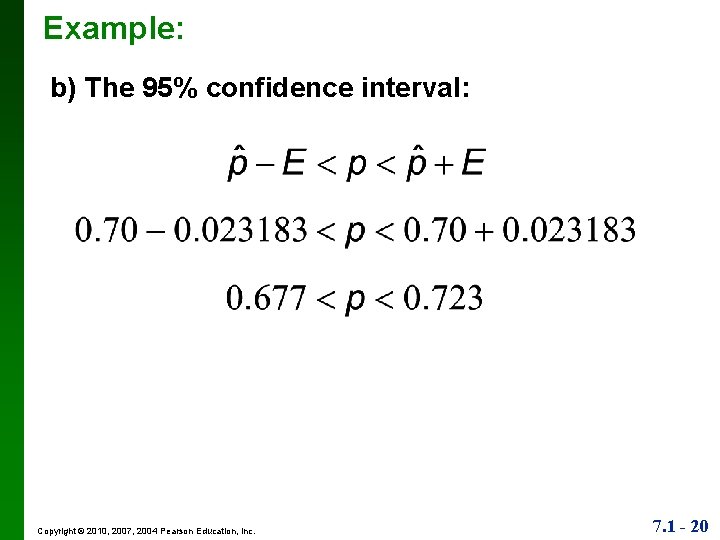
Example: b) The 95% confidence interval: Copyright © 2010, 2007, 2004 Pearson Education, Inc. 7. 1 - 20

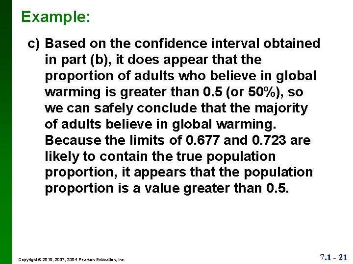
Example: c) Based on the confidence interval obtained in part (b), it does appear that the proportion of adults who believe in global warming is greater than 0. 5 (or 50%), so we can safely conclude that the majority of adults believe in global warming. Because the limits of 0. 677 and 0. 723 are likely to contain the true population proportion, it appears that the population proportion is a value greater than 0. 5. Copyright © 2010, 2007, 2004 Pearson Education, Inc. 7. 1 - 21

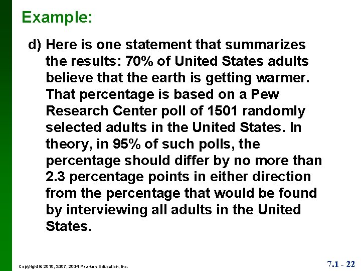
Example: d) Here is one statement that summarizes the results: 70% of United States adults believe that the earth is getting warmer. That percentage is based on a Pew Research Center poll of 1501 randomly selected adults in the United States. In theory, in 95% of such polls, the percentage should differ by no more than 2. 3 percentage points in either direction from the percentage that would be found by interviewing all adults in the United States. Copyright © 2010, 2007, 2004 Pearson Education, Inc. 7. 1 - 22

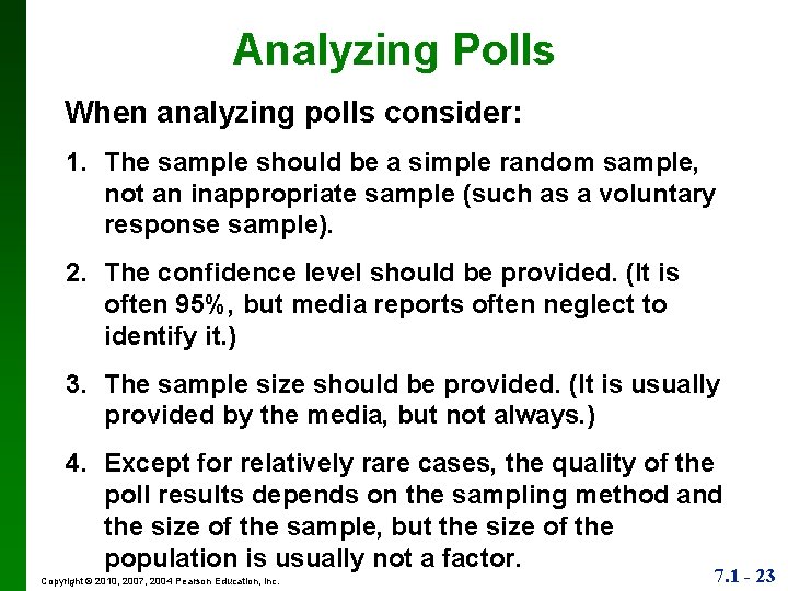
Analyzing Polls When analyzing polls consider: 1. The sample should be a simple random sample, not an inappropriate sample (such as a voluntary response sample). 2. The confidence level should be provided. (It is often 95%, but media reports often neglect to identify it. ) 3. The sample size should be provided. (It is usually provided by the media, but not always. ) 4. Except for relatively rare cases, the quality of the poll results depends on the sampling method and the size of the sample, but the size of the population is usually not a factor. Copyright © 2010, 2007, 2004 Pearson Education, Inc. 7. 1 - 23

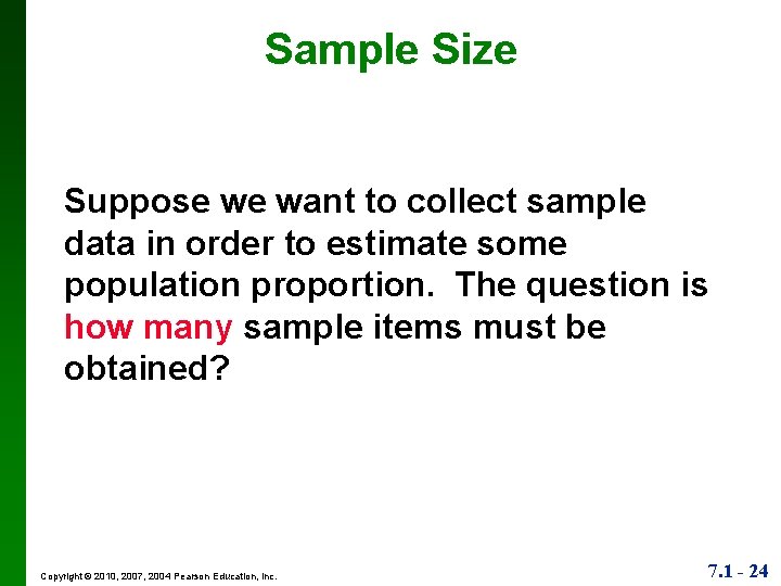
Sample Size Suppose we want to collect sample data in order to estimate some population proportion. The question is how many sample items must be obtained? Copyright © 2010, 2007, 2004 Pearson Education, Inc. 7. 1 - 24

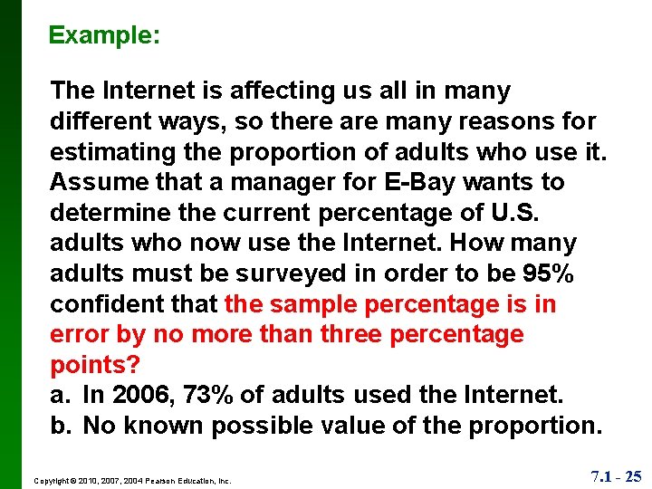
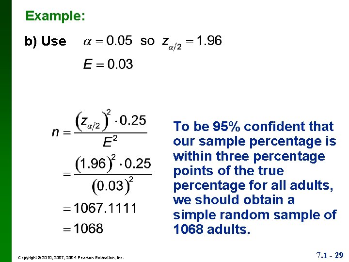
Example: The Internet is affecting us all in many different ways, so there are many reasons for estimating the proportion of adults who use it. Assume that a manager for E-Bay wants to determine the current percentage of U. S. adults who now use the Internet. How many adults must be surveyed in order to be 95% confident that the sample percentage is in error by no more than three percentage points? a. In 2006, 73% of adults used the Internet. b. No known possible value of the proportion. Copyright © 2010, 2007, 2004 Pearson Education, Inc. 7. 1 - 25

Sample Size for Estimating Proportion p Copyright © 2010, 2007, 2004 Pearson Education, Inc. 7. 1 - 26

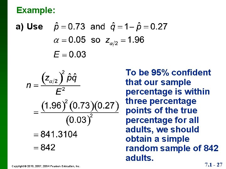
Example: a) Use To be 95% confident that our sample percentage is within three percentage points of the true percentage for all adults, we should obtain a simple random sample of 842 adults. Copyright © 2010, 2007, 2004 Pearson Education, Inc. 7. 1 - 27

Round-Off Rule for Determining Sample Size If the computed sample size n is not a whole number, round the value of n up to the next larger whole number. Copyright © 2010, 2007, 2004 Pearson Education, Inc. 7. 1 - 28

Example: b) Use To be 95% confident that our sample percentage is within three percentage points of the true percentage for all adults, we should obtain a simple random sample of 1068 adults. Copyright © 2010, 2007, 2004 Pearson Education, Inc. 7. 1 - 29

Section 7 -3 Estimating a Population Mean: σ Known Copyright © 2010, 2007, 2004 Pearson Education, Inc. 7. 1 - 30

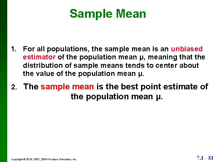
Sample Mean 1. For all populations, the sample mean is an unbiased estimator of the population mean μ, meaning that the distribution of sample means tends to center about the value of the population mean μ. 2. The sample mean is the best point estimate of the population mean μ. Copyright © 2010, 2007, 2004 Pearson Education, Inc. 7. 1 - 31

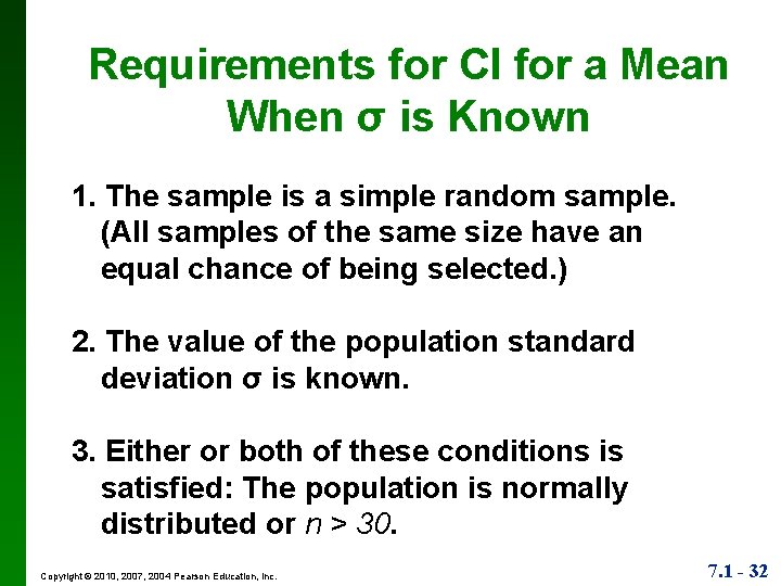
Requirements for CI for a Mean When σ is Known 1. The sample is a simple random sample. (All samples of the same size have an equal chance of being selected. ) 2. The value of the population standard deviation σ is known. 3. Either or both of these conditions is satisfied: The population is normally distributed or n > 30. Copyright © 2010, 2007, 2004 Pearson Education, Inc. 7. 1 - 32

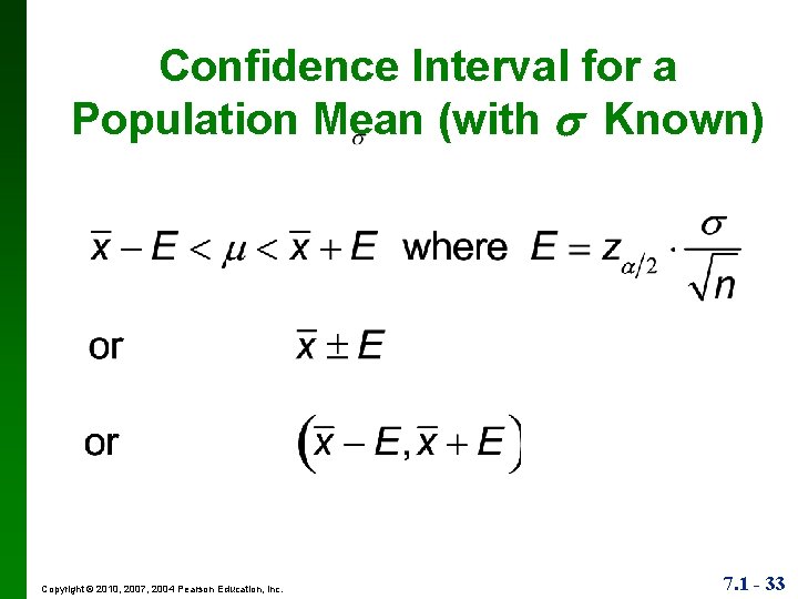
Confidence Interval for a Population Mean (with Known) Copyright © 2010, 2007, 2004 Pearson Education, Inc. 7. 1 - 33

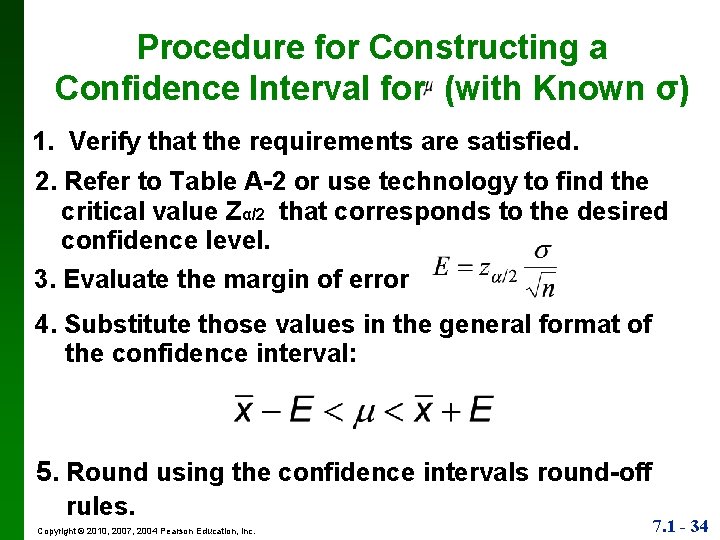
Procedure for Constructing a Confidence Interval for (with Known σ) 1. Verify that the requirements are satisfied. 2. Refer to Table A-2 or use technology to find the critical value Zα/2 that corresponds to the desired confidence level. 3. Evaluate the margin of error 4. Substitute those values in the general format of the confidence interval: 5. Round using the confidence intervals round-off rules. Copyright © 2010, 2007, 2004 Pearson Education, Inc. 7. 1 - 34

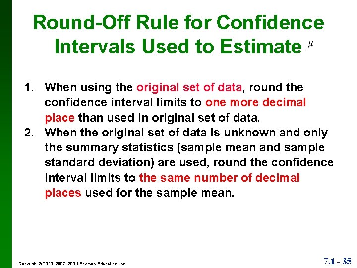
Round-Off Rule for Confidence Intervals Used to Estimate 1. When using the original set of data, round the confidence interval limits to one more decimal place than used in original set of data. 2. When the original set of data is unknown and only the summary statistics (sample mean and sample standard deviation) are used, round the confidence interval limits to the same number of decimal places used for the sample mean. Copyright © 2010, 2007, 2004 Pearson Education, Inc. 7. 1 - 35

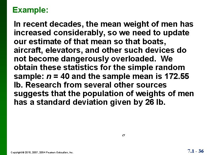
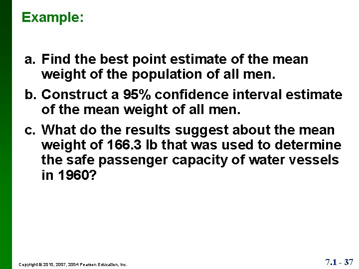
Example: In recent decades, the mean weight of men has increased considerably, so we need to update our estimate of that mean so that boats, aircraft, elevators, and other such devices do not become dangerously overloaded. We obtain these statistics for the simple random sample: n = 40 and the sample mean is 172. 55 lb. Research from several other sources suggests that the population of weights of men has a standard deviation given by 26 lb. Copyright © 2010, 2007, 2004 Pearson Education, Inc. 7. 1 - 36

Example: a. Find the best point estimate of the mean weight of the population of all men. b. Construct a 95% confidence interval estimate of the mean weight of all men. c. What do the results suggest about the mean weight of 166. 3 lb that was used to determine the safe passenger capacity of water vessels in 1960? Copyright © 2010, 2007, 2004 Pearson Education, Inc. 7. 1 - 37

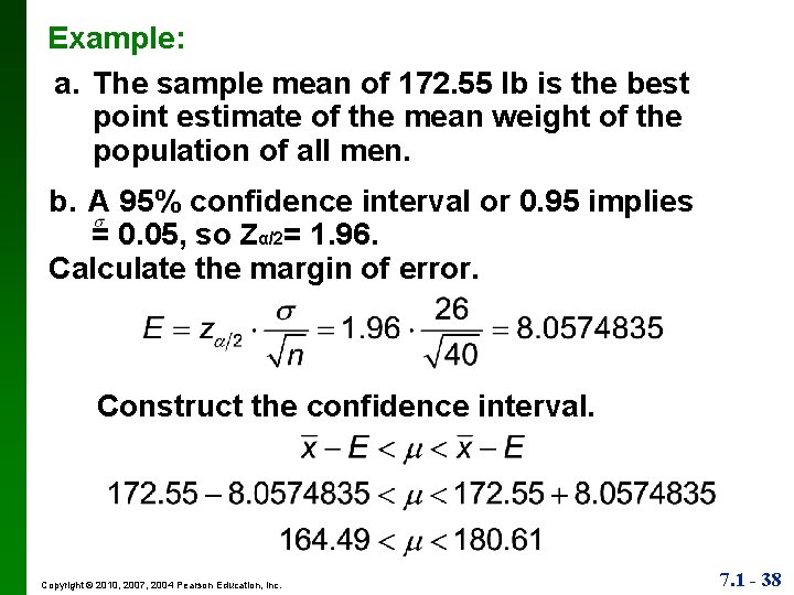
Example: a. The sample mean of 172. 55 lb is the best point estimate of the mean weight of the population of all men. b. A 95% confidence interval or 0. 95 implies = 0. 05, so Zα/2= 1. 96. Calculate the margin of error. Construct the confidence interval. Copyright © 2010, 2007, 2004 Pearson Education, Inc. 7. 1 - 38

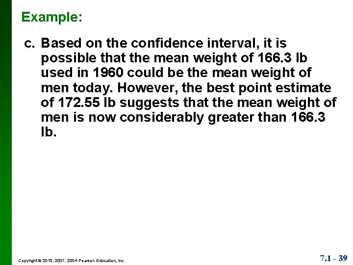
Example: c. Based on the confidence interval, it is possible that the mean weight of 166. 3 lb used in 1960 could be the mean weight of men today. However, the best point estimate of 172. 55 lb suggests that the mean weight of men is now considerably greater than 166. 3 lb. Copyright © 2010, 2007, 2004 Pearson Education, Inc. 7. 1 - 39

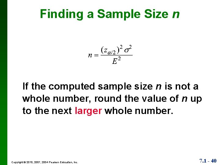
Finding a Sample Size n If the computed sample size n is not a whole number, round the value of n up to the next larger whole number. Copyright © 2010, 2007, 2004 Pearson Education, Inc. 7. 1 - 40

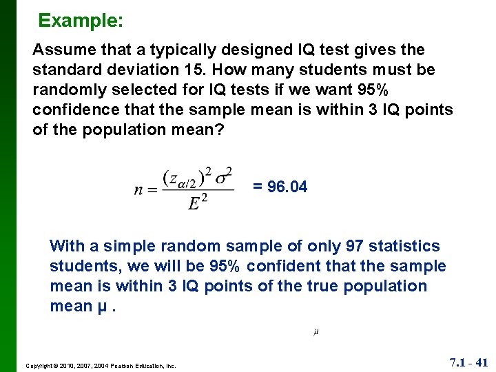
Example: Assume that a typically designed IQ test gives the standard deviation 15. How many students must be randomly selected for IQ tests if we want 95% confidence that the sample mean is within 3 IQ points of the population mean? = 96. 04 With a simple random sample of only 97 statistics students, we will be 95% confident that the sample mean is within 3 IQ points of the true population mean μ. Copyright © 2010, 2007, 2004 Pearson Education, Inc. 7. 1 - 41

Section 7 -4 Estimating a Population Mean: σ Not Known Copyright © 2010, 2007, 2004 Pearson Education, Inc. 7. 1 - 42

Student t Distribution This section presents methods for estimating a population mean when the population standard deviation is not known. With unknown, we use the Student t distribution assuming that the relevant requirements are satisfied. Copyright © 2010, 2007, 2004 Pearson Education, Inc. 7. 1 - 43

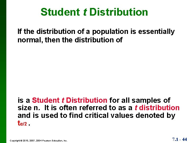
Student t Distribution If the distribution of a population is essentially normal, then the distribution of is a Student t Distribution for all samples of size n. It is often referred to as a t distribution and is used to find critical values denoted by tα/2. Copyright © 2010, 2007, 2004 Pearson Education, Inc. 7. 1 - 44

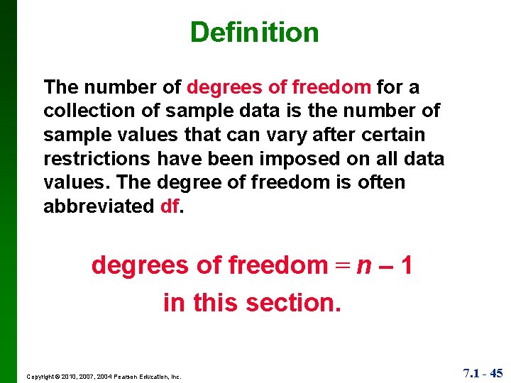
Definition The number of degrees of freedom for a collection of sample data is the number of sample values that can vary after certain restrictions have been imposed on all data values. The degree of freedom is often abbreviated df. degrees of freedom = n – 1 in this section. Copyright © 2010, 2007, 2004 Pearson Education, Inc. 7. 1 - 45

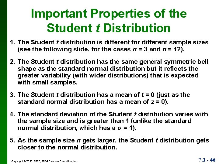
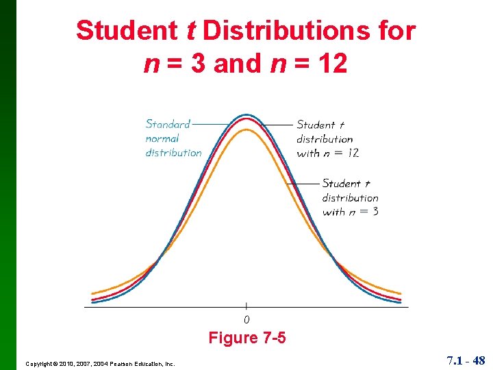
Important Properties of the Student t Distribution 1. The Student t distribution is different for different sample sizes (see the following slide, for the cases n = 3 and n = 12). 2. The Student t distribution has the same general symmetric bell shape as the standard normal distribution but it reflects the greater variability (with wider distributions) that is expected with small samples. 3. The Student t distribution has a mean of t = 0 (just as the standard normal distribution has a mean of z = 0). 4. The standard deviation of the Student t distribution varies with the sample size and is greater than 1 (unlike the standard normal distribution, which has a σ = 1). 5. As the sample size n gets larger, the Student t distribution gets closer to the normal distribution. Copyright © 2010, 2007, 2004 Pearson Education, Inc. 7. 1 - 46

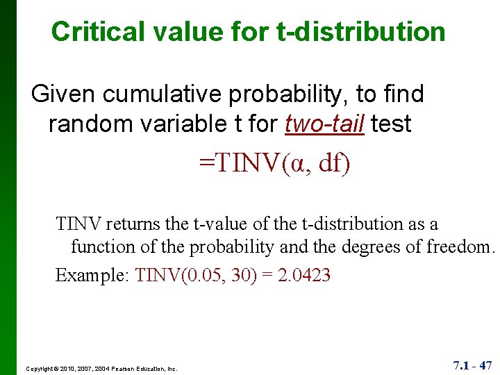
Critical value for t-distribution Given cumulative probability, to find random variable t for two-tail test =TINV(α, df) TINV returns the t-value of the t-distribution as a function of the probability and the degrees of freedom. Example: TINV(0. 05, 30) = 2. 0423 Copyright © 2010, 2007, 2004 Pearson Education, Inc. 7. 1 - 47

Student t Distributions for n = 3 and n = 12 Figure 7 -5 Copyright © 2010, 2007, 2004 Pearson Education, Inc. 7. 1 - 48

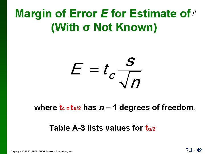
Margin of Error E for Estimate of (With σ Not Known) where tc = tα/2 has n – 1 degrees of freedom. Table A-3 lists values for tα/2 Copyright © 2010, 2007, 2004 Pearson Education, Inc. 7. 1 - 49

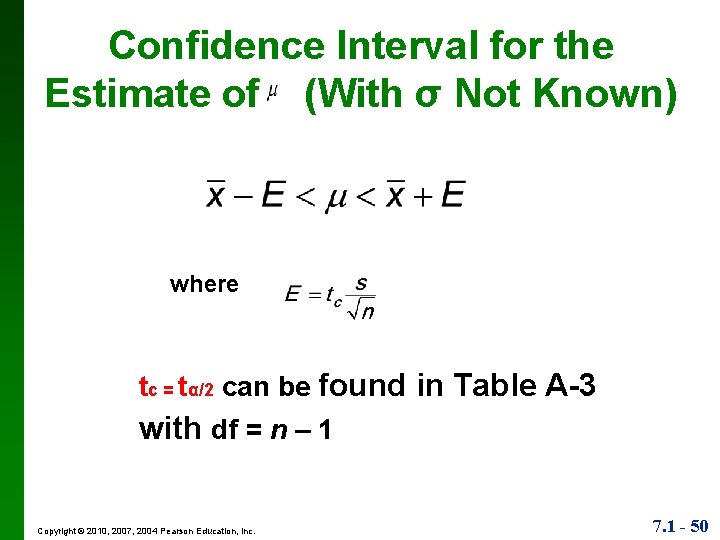
Confidence Interval for the Estimate of (With σ Not Known) where tc = tα/2 can be found in Table A-3 with df = n – 1 Copyright © 2010, 2007, 2004 Pearson Education, Inc. 7. 1 - 50

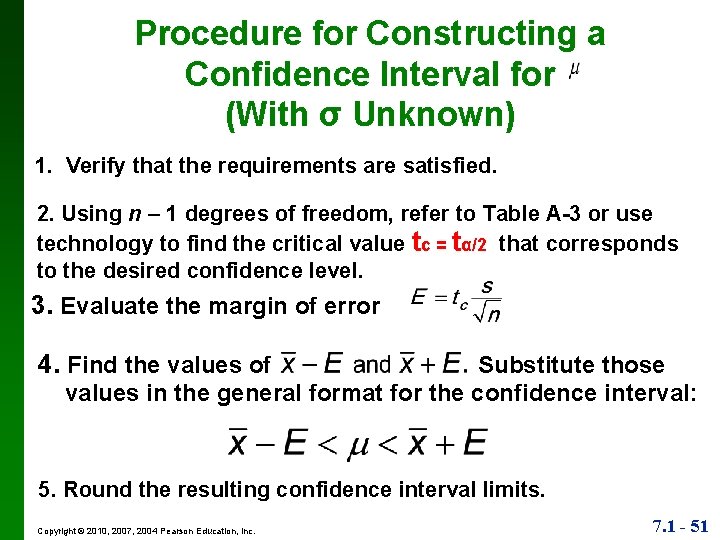
Procedure for Constructing a Confidence Interval for (With σ Unknown) 1. Verify that the requirements are satisfied. 2. Using n – 1 degrees of freedom, refer to Table A-3 or use technology to find the critical value tc = tα/2 that corresponds to the desired confidence level. 3. Evaluate the margin of error 4. Find the values of Substitute those values in the general format for the confidence interval: 5. Round the resulting confidence interval limits. Copyright © 2010, 2007, 2004 Pearson Education, Inc. 7. 1 - 51

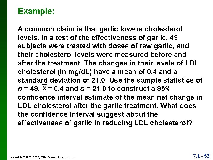
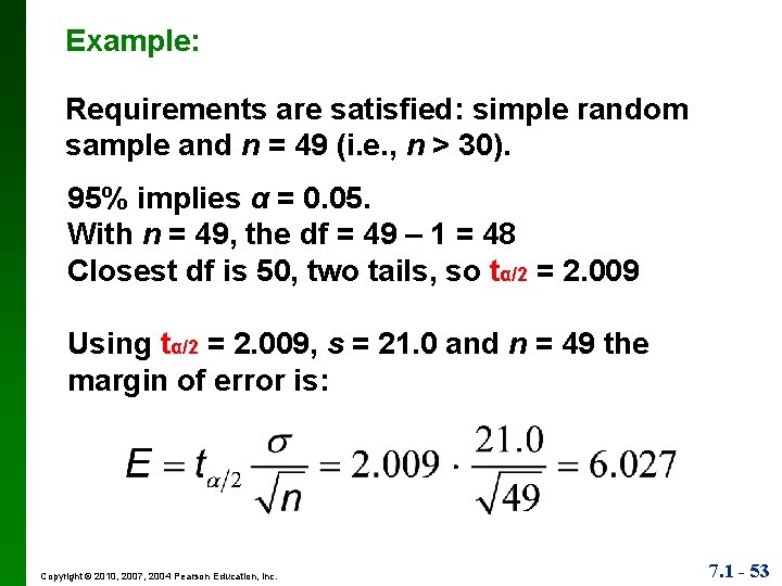
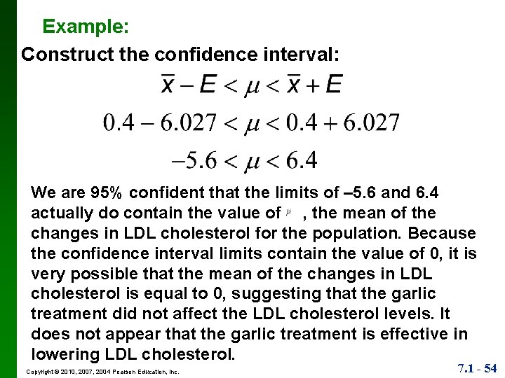
Example: A common claim is that garlic lowers cholesterol levels. In a test of the effectiveness of garlic, 49 subjects were treated with doses of raw garlic, and their cholesterol levels were measured before and after the treatment. The changes in their levels of LDL cholesterol (in mg/d. L) have a mean of 0. 4 and a standard deviation of 21. 0. Use the sample statistics of n = 49, = 0. 4 and s = 21. 0 to construct a 95% confidence interval estimate of the mean net change in LDL cholesterol after the garlic treatment. What does the confidence interval suggest about the effectiveness of garlic in reducing LDL cholesterol? Copyright © 2010, 2007, 2004 Pearson Education, Inc. 7. 1 - 52

Example: Requirements are satisfied: simple random sample and n = 49 (i. e. , n > 30). 95% implies α = 0. 05. With n = 49, the df = 49 – 1 = 48 Closest df is 50, two tails, so tα/2 = 2. 009 Using tα/2 = 2. 009, s = 21. 0 and n = 49 the margin of error is: Copyright © 2010, 2007, 2004 Pearson Education, Inc. 7. 1 - 53

Example: Construct the confidence interval: We are 95% confident that the limits of – 5. 6 and 6. 4 actually do contain the value of , the mean of the changes in LDL cholesterol for the population. Because the confidence interval limits contain the value of 0, it is very possible that the mean of the changes in LDL cholesterol is equal to 0, suggesting that the garlic treatment did not affect the LDL cholesterol levels. It does not appear that the garlic treatment is effective in lowering LDL cholesterol. Copyright © 2010, 2007, 2004 Pearson Education, Inc. 7. 1 - 54

Section 7 -5 Estimating a Population Variance Copyright © 2010, 2007, 2004 Pearson Education, Inc. 7. 1 - 55

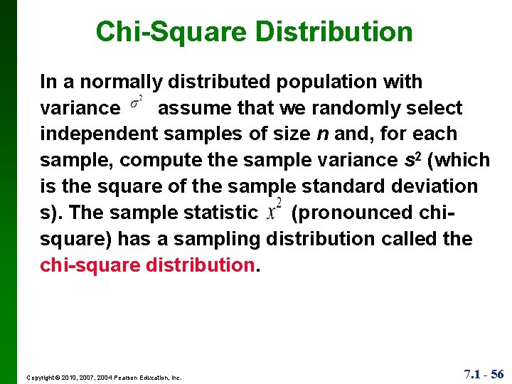
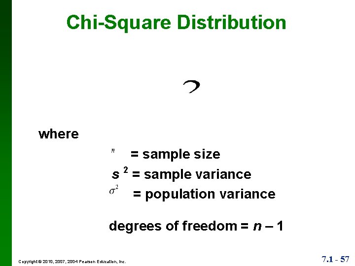
Chi-Square Distribution In a normally distributed population with variance assume that we randomly select independent samples of size n and, for each sample, compute the sample variance s 2 (which is the square of the sample standard deviation s). The sample statistic (pronounced chisquare) has a sampling distribution called the chi-square distribution. Copyright © 2010, 2007, 2004 Pearson Education, Inc. 7. 1 - 56

Chi-Square Distribution where = sample size s 2 = sample variance = population variance degrees of freedom = n – 1 Copyright © 2010, 2007, 2004 Pearson Education, Inc. 7. 1 - 57

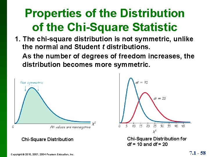
Properties of the Distribution of the Chi-Square Statistic 1. The chi-square distribution is not symmetric, unlike the normal and Student t distributions. As the number of degrees of freedom increases, the distribution becomes more symmetric. Chi-Square Distribution Copyright © 2010, 2007, 2004 Pearson Education, Inc. Chi-Square Distribution for df = 10 and df = 20 7. 1 - 58

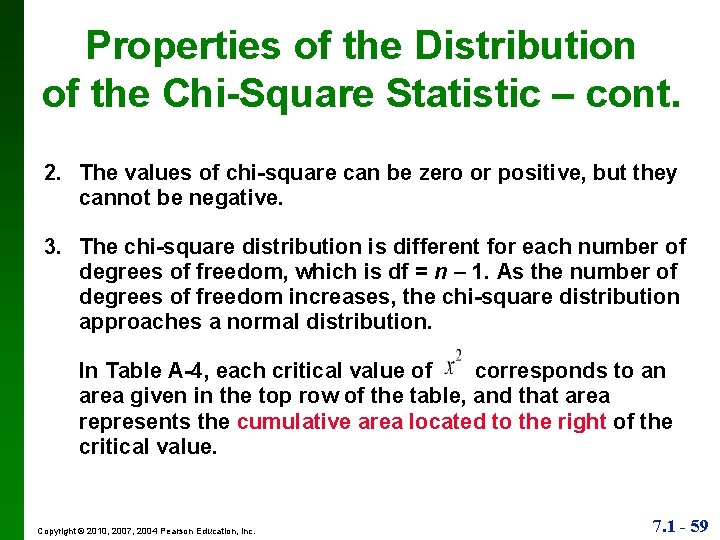
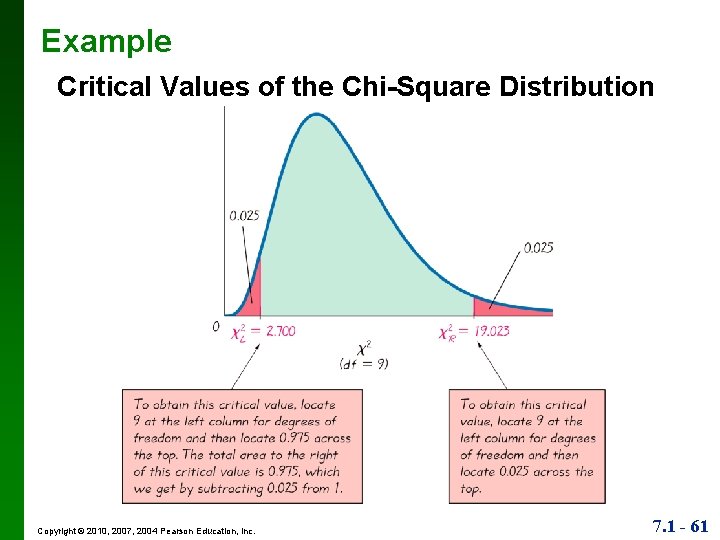
Properties of the Distribution of the Chi-Square Statistic – cont. 2. The values of chi-square can be zero or positive, but they cannot be negative. 3. The chi-square distribution is different for each number of degrees of freedom, which is df = n – 1. As the number of degrees of freedom increases, the chi-square distribution approaches a normal distribution. In Table A-4, each critical value of corresponds to an area given in the top row of the table, and that area represents the cumulative area located to the right of the critical value. Copyright © 2010, 2007, 2004 Pearson Education, Inc. 7. 1 - 59

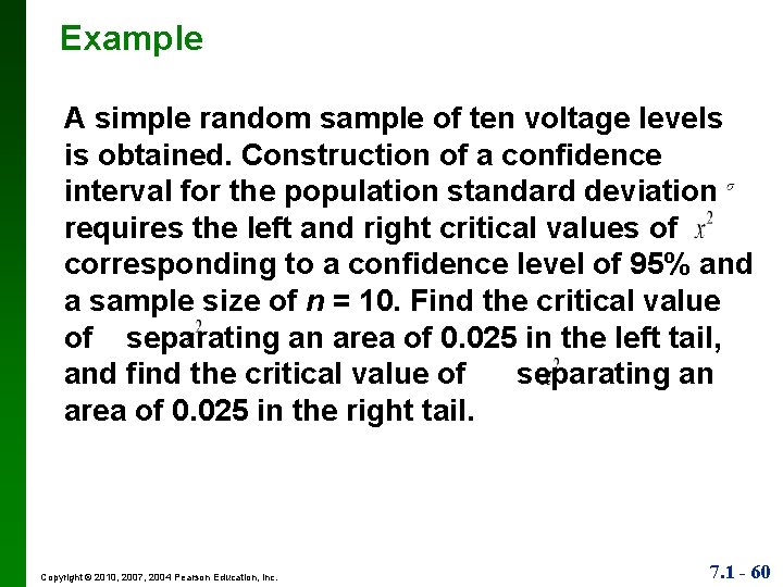
Example A simple random sample of ten voltage levels is obtained. Construction of a confidence interval for the population standard deviation requires the left and right critical values of corresponding to a confidence level of 95% and a sample size of n = 10. Find the critical value of separating an area of 0. 025 in the left tail, and find the critical value of separating an area of 0. 025 in the right tail. Copyright © 2010, 2007, 2004 Pearson Education, Inc. 7. 1 - 60

Example Critical Values of the Chi-Square Distribution Copyright © 2010, 2007, 2004 Pearson Education, Inc. 7. 1 - 61

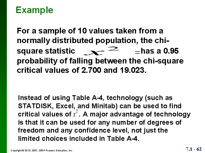
Example For a sample of 10 values taken from a normally distributed population, the chisquare statistic has a 0. 95 probability of falling between the chi-square critical values of 2. 700 and 19. 023. Instead of using Table A-4, technology (such as STATDISK, Excel, and Minitab) can be used to find critical values of. A major advantage of technology is that it can be used for any number of degrees of freedom and any confidence level, not just the limited choices included in Table A-4. Copyright © 2010, 2007, 2004 Pearson Education, Inc. 7. 1 - 62

Estimators of The sample variance s 2 is the best point estimate of the population variance. Copyright © 2010, 2007, 2004 Pearson Education, Inc. 7. 1 - 63

Estimators of The sample standard deviation s is a commonly used point estimate of (even though it is a biased estimate). Copyright © 2010, 2007, 2004 Pearson Education, Inc. 7. 1 - 64

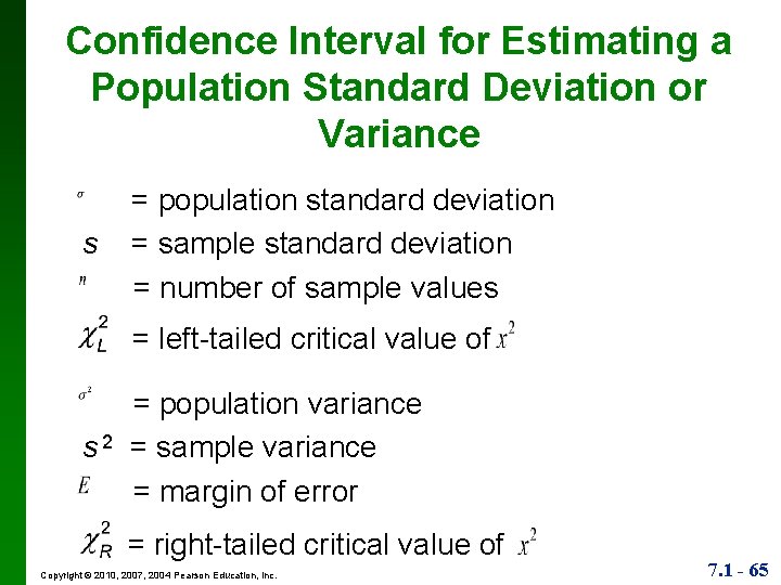
Confidence Interval for Estimating a Population Standard Deviation or Variance s = population standard deviation = sample standard deviation = number of sample values = left-tailed critical value of s 2 = population variance = sample variance = margin of error = right-tailed critical value of Copyright © 2010, 2007, 2004 Pearson Education, Inc. 7. 1 - 65

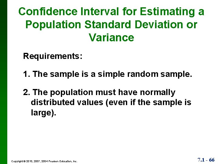
Confidence Interval for Estimating a Population Standard Deviation or Variance Requirements: 1. The sample is a simple random sample. 2. The population must have normally distributed values (even if the sample is large). Copyright © 2010, 2007, 2004 Pearson Education, Inc. 7. 1 - 66

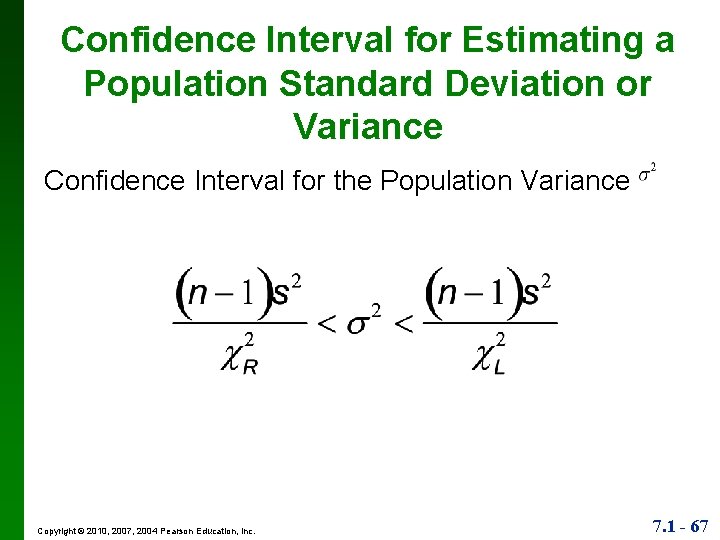
Confidence Interval for Estimating a Population Standard Deviation or Variance Confidence Interval for the Population Variance Copyright © 2010, 2007, 2004 Pearson Education, Inc. 7. 1 - 67

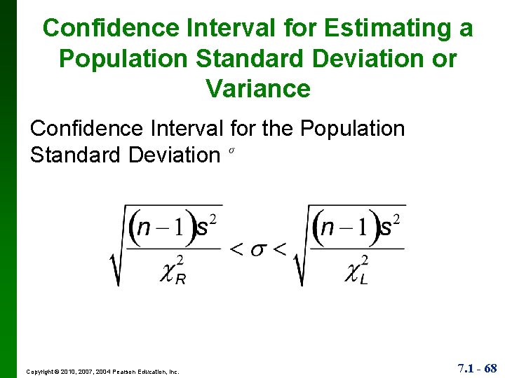
Confidence Interval for Estimating a Population Standard Deviation or Variance Confidence Interval for the Population Standard Deviation Copyright © 2010, 2007, 2004 Pearson Education, Inc. 7. 1 - 68

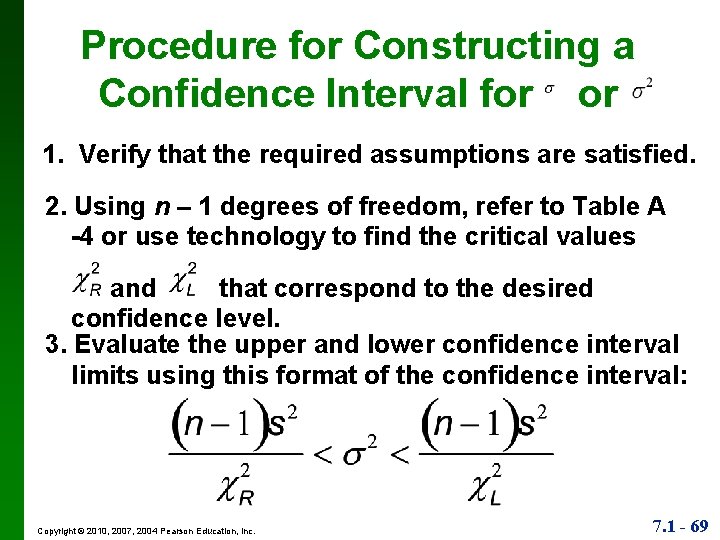
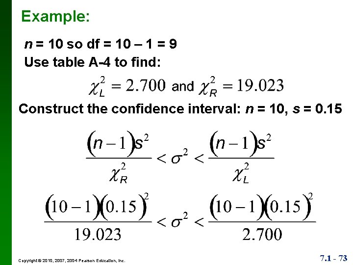
Procedure for Constructing a Confidence Interval for or 1. Verify that the required assumptions are satisfied. 2. Using n – 1 degrees of freedom, refer to Table A -4 or use technology to find the critical values and that correspond to the desired confidence level. 3. Evaluate the upper and lower confidence interval limits using this format of the confidence interval: Copyright © 2010, 2007, 2004 Pearson Education, Inc. 7. 1 - 69

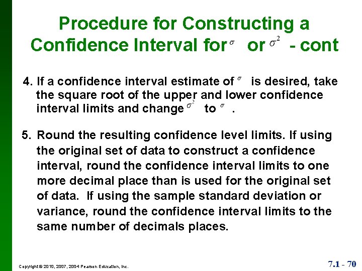
Procedure for Constructing a Confidence Interval for or - cont 4. If a confidence interval estimate of is desired, take the square root of the upper and lower confidence interval limits and change to. 5. Round the resulting confidence level limits. If using the original set of data to construct a confidence interval, round the confidence interval limits to one more decimal place than is used for the original set of data. If using the sample standard deviation or variance, round the confidence interval limits to the same number of decimals places. Copyright © 2010, 2007, 2004 Pearson Education, Inc. 7. 1 - 70

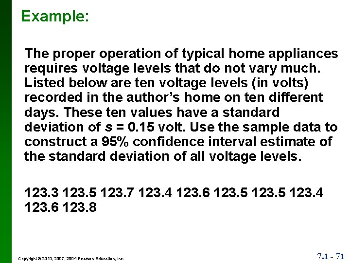
Example: The properation of typical home appliances requires voltage levels that do not vary much. Listed below are ten voltage levels (in volts) recorded in the author’s home on ten different days. These ten values have a standard deviation of s = 0. 15 volt. Use the sample data to construct a 95% confidence interval estimate of the standard deviation of all voltage levels. 123. 3 123. 5 123. 7 123. 4 123. 6 123. 5 123. 4 123. 6 123. 8 Copyright © 2010, 2007, 2004 Pearson Education, Inc. 7. 1 - 71

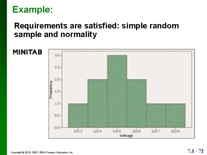
Example: Requirements are satisfied: simple random sample and normality Copyright © 2010, 2007, 2004 Pearson Education, Inc. 7. 1 - 72

Example: n = 10 so df = 10 – 1 = 9 Use table A-4 to find: Construct the confidence interval: n = 10, s = 0. 15 Copyright © 2010, 2007, 2004 Pearson Education, Inc. 7. 1 - 73

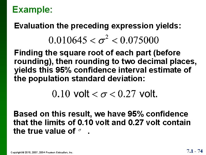
Example: Evaluation the preceding expression yields: Finding the square root of each part (before rounding), then rounding to two decimal places, yields this 95% confidence interval estimate of the population standard deviation: Based on this result, we have 95% confidence that the limits of 0. 10 volt and 0. 27 volt contain the true value of . Copyright © 2010, 2007, 2004 Pearson Education, Inc. 7. 1 - 74

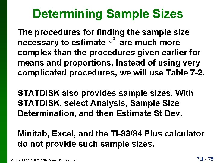
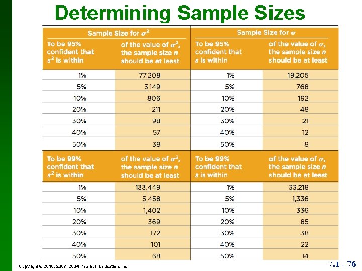
Determining Sample Sizes The procedures for finding the sample size necessary to estimate are much more complex than the procedures given earlier for means and proportions. Instead of using very complicated procedures, we will use Table 7 -2. STATDISK also provides sample sizes. With STATDISK, select Analysis, Sample Size Determination, and then Estimate St Dev. Minitab, Excel, and the TI-83/84 Plus calculator do not provide such sample sizes. Copyright © 2010, 2007, 2004 Pearson Education, Inc. 7. 1 - 75

Determining Sample Sizes Copyright © 2010, 2007, 2004 Pearson Education, Inc. 7. 1 - 76

Example: We want to estimate the standard deviation σ of all voltage levels in a home. We want to be 95% confident that our estimate is within 20% of the true value of σ. How large should the sample be? Assume that the population is normally distributed. Copyright © 2010, 2007, 2004 Pearson Education, Inc. 7. 1 - 77