Estimating a population proportion ASW 6 3 7

Estimating a population proportion ASW, 6. 3, 7. 6, 8. 4 Economics 224 notes for October 20, 2008

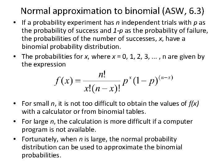
Normal approximation to binomial (ASW, 6. 3) • If a probability experiment has n independent trials with p as the probability of success and 1 -p as the probability of failure, the probabilities of the number of successes, x, have a binomial probability distribution. • The probabilities for x, where x = 0, 1, 2, 3, . . . , n are given by the expression • For small n, it is not too difficult to obtain the values of f(x) with a calculator or from binomial tables. • For large n, the calculation is more difficult if a computer program is not available. • Fortunately, when n is large, the normal probability distribution can be used to approximate the binomial probabilities.

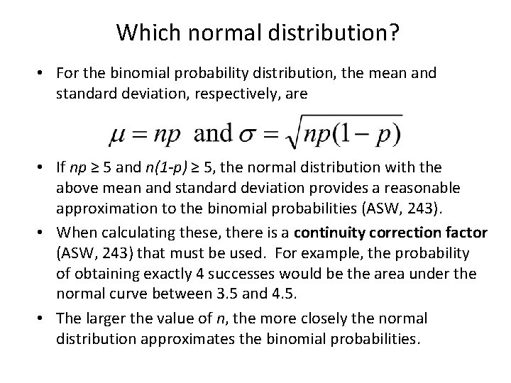
Which normal distribution? • For the binomial probability distribution, the mean and standard deviation, respectively, are • If np ≥ 5 and n(1 -p) ≥ 5, the normal distribution with the above mean and standard deviation provides a reasonable approximation to the binomial probabilities (ASW, 243). • When calculating these, there is a continuity correction factor (ASW, 243) that must be used. For example, the probability of obtaining exactly 4 successes would be the area under the normal curve between 3. 5 and 4. 5. • The larger the value of n, the more closely the normal distribution approximates the binomial probabilities.

Population proportion p • When conducting research about a population, researchers are often more interested in the proportion of a population with a particular characteristic, rather than the number of population elements with the characteristic. – – Proportion of population who support the Liberals. Proportion of manufactured objects that are defect free. Proportion of employees with extended health care plans. Percentage of the labour force that is unemployed. • In each of these situations, the actual number of population elements with the characteristic will vary with the sample size. But the aim of obtaining samples is to estimate the proportion, or percentage, of the population with the characteristic. • Let the proportion of a population with a particular characteristics be represented by p.

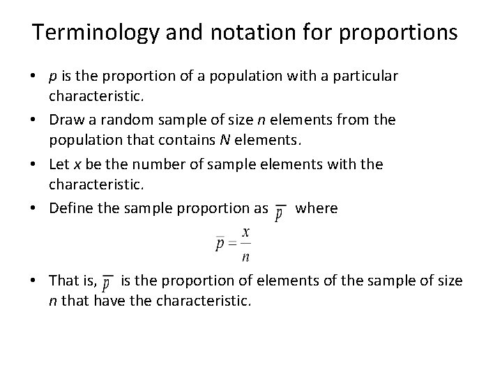
Terminology and notation for proportions • p is the proportion of a population with a particular characteristic. • Draw a random sample of size n elements from the population that contains N elements. • Let x be the number of sample elements with the characteristic. • Define the sample proportion as where • That is, is the proportion of elements of the sample of size n that have the characteristic.

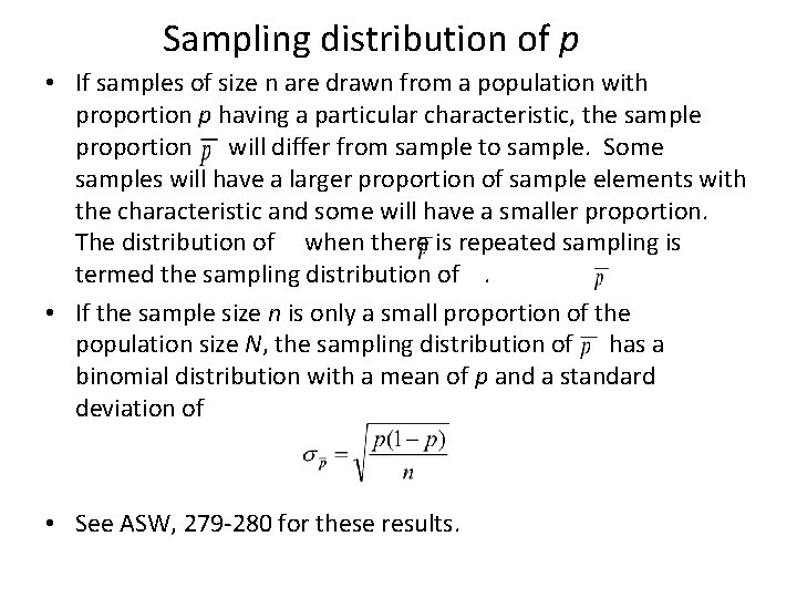
Sampling distribution of p • If samples of size n are drawn from a population with proportion p having a particular characteristic, the sample proportion will differ from sample to sample. Some samples will have a larger proportion of sample elements with the characteristic and some will have a smaller proportion. The distribution of when there is repeated sampling is termed the sampling distribution of. • If the sample size n is only a small proportion of the population size N, the sampling distribution of has a binomial distribution with a mean of p and a standard deviation of • See ASW, 279 -280 for these results.

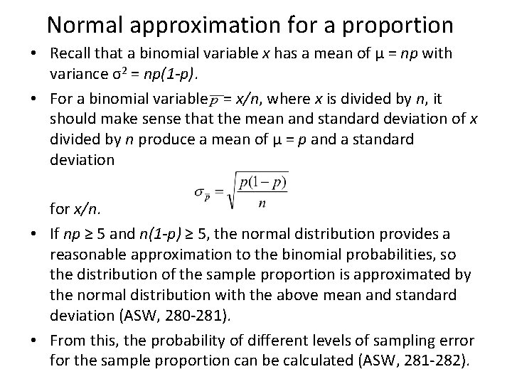
Normal approximation for a proportion • Recall that a binomial variable x has a mean of μ = np with variance σ2 = np(1 -p). • For a binomial variable = x/n, where x is divided by n, it should make sense that the mean and standard deviation of x divided by n produce a mean of μ = p and a standard deviation for x/n. • If np ≥ 5 and n(1 -p) ≥ 5, the normal distribution provides a reasonable approximation to the binomial probabilities, so the distribution of the sample proportion is approximated by the normal distribution with the above mean and standard deviation (ASW, 280 -281). • From this, the probability of different levels of sampling error for the sample proportion can be calculated (ASW, 281 -282).

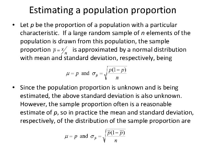
Estimating a population proportion • Let p be the proportion of a population with a particular characteristic. If a large random sample of n elements of the population is drawn from this population, the sample proportion is approximated by a normal distribution with mean and standard deviation, respectively, being • Since the population proportion is unknown and is being estimated, the above standard deviation is also unknown. However, the sample proportion often is a reasonable estimate of p, so in practice the mean and standard deviation, respectively, of the distribution of the sample proportion are

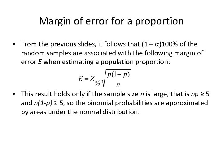
Margin of error for a proportion • From the previous slides, it follows that (1 – α)100% of the random samples are associated with the following margin of error E when estimating a population proportion: • This result holds only if the sample size n is large, that is np ≥ 5 and n(1 -p) ≥ 5, so the binomial probabilities are approximated by areas under the normal distribution.

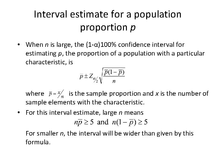
Interval estimate for a population proportion p • When n is large, the (1 -α)100% confidence interval for estimating p, the proportion of a population with a particular characteristic, is where is the sample proportion and x is the number of sample elements with the characteristic. • For this interval estimate, large n means For smaller n, the interval will be wider than given by this formula.

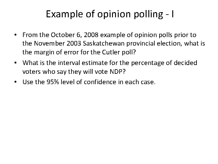
Example of opinion polling - I • From the October 6, 2008 example of opinion polls prior to the November 2003 Saskatchewan provincial election, what is the margin of error for the Cutler poll? • What is the interval estimate for the percentage of decided voters who say they will vote NDP? • Use the 95% level of confidence in each case.

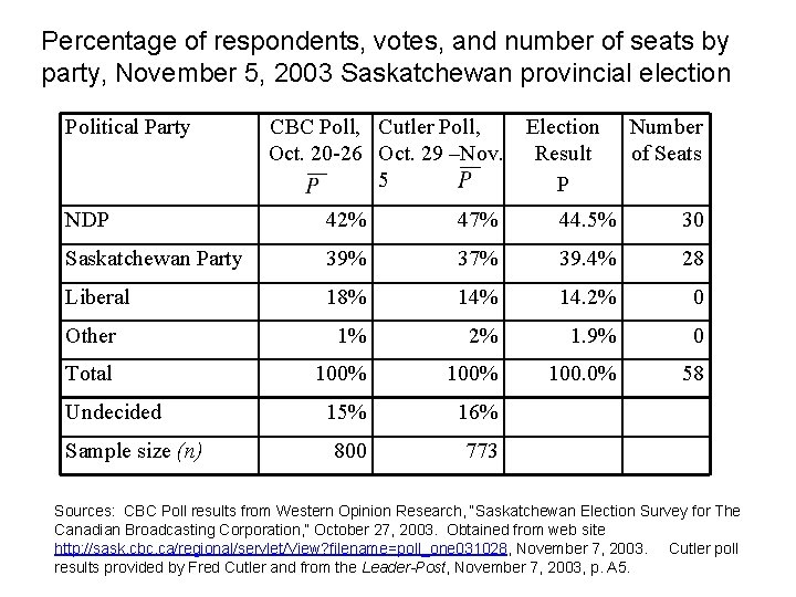
Percentage of respondents, votes, and number of seats by party, November 5, 2003 Saskatchewan provincial election Political Party CBC Poll, Cutler Poll, Oct. 20 -26 Oct. 29 –Nov. 5 Election Result P Number of Seats NDP 42% 47% 44. 5% 30 Saskatchewan Party 39% 37% 39. 4% 28 Liberal 18% 14. 2% 0 Other 1% 2% 1. 9% 0 Total 100% 100. 0% 58 15% 16% 800 773 Undecided Sample size (n) Sources: CBC Poll results from Western Opinion Research, “Saskatchewan Election Survey for The Canadian Broadcasting Corporation, ” October 27, 2003. Obtained from web site http: //sask. cbc. ca/regional/servlet/View? filename=poll_one 031028, November 7, 2003. Cutler poll results provided by Fred Cutler and from the Leader-Post, November 7, 2003, p. A 5.

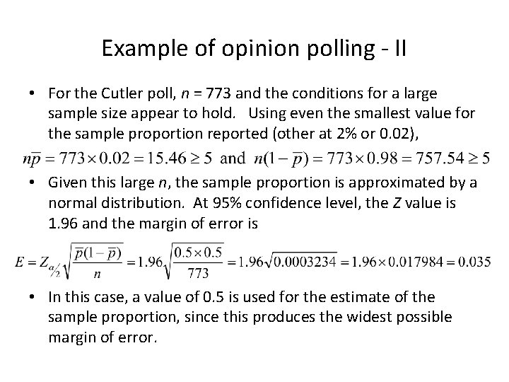
Example of opinion polling - II • For the Cutler poll, n = 773 and the conditions for a large sample size appear to hold. Using even the smallest value for the sample proportion reported (other at 2% or 0. 02), • Given this large n, the sample proportion is approximated by a normal distribution. At 95% confidence level, the Z value is 1. 96 and the margin of error is • In this case, a value of 0. 5 is used for the estimate of the sample proportion, since this produces the widest possible margin of error.

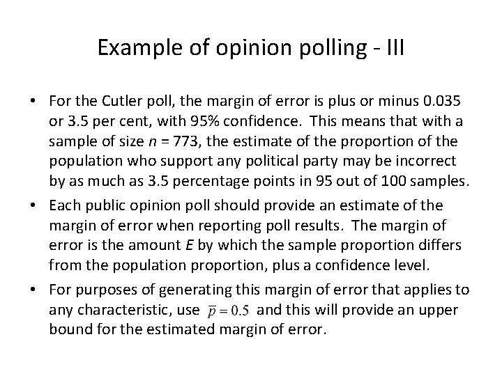
Example of opinion polling - III • For the Cutler poll, the margin of error is plus or minus 0. 035 or 3. 5 per cent, with 95% confidence. This means that with a sample of size n = 773, the estimate of the proportion of the population who support any political party may be incorrect by as much as 3. 5 percentage points in 95 out of 100 samples. • Each public opinion poll should provide an estimate of the margin of error when reporting poll results. The margin of error is the amount E by which the sample proportion differs from the population proportion, plus a confidence level. • For purposes of generating this margin of error that applies to any characteristic, use and this will provide an upper bound for the estimated margin of error.

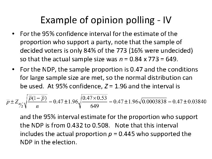
Example of opinion polling - IV • For the 95% confidence interval for the estimate of the proportion who support a party, note that the sample of decided voters is only 84% of the 773 (16% were undecided) so that the actual sample size was n = 0. 84 x 773 = 649. • For the NDP, the sample proportion is 0. 47 and the conditions for large sample size are met, so the normal distribution can be used. At 95% confidence, Z = 1. 96 and the interval is and the 95% interval estimate for the proportion who support the NDP is from 0. 432 to 0. 508. Note that this interval includes the actual proportion p = 0. 445 who supported the NDP in the election.

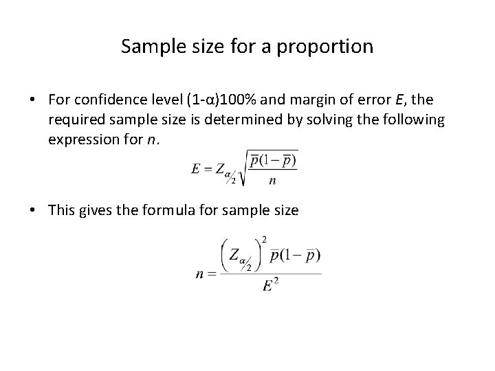
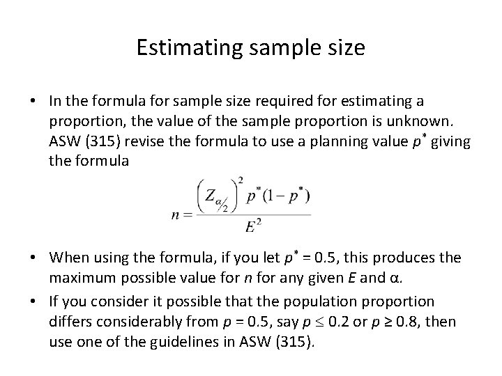
Sample size for a proportion • For confidence level (1 -α)100% and margin of error E, the required sample size is determined by solving the following expression for n. • This gives the formula for sample size

Estimating sample size • In the formula for sample size required for estimating a proportion, the value of the sample proportion is unknown. ASW (315) revise the formula to use a planning value p* giving the formula • When using the formula, if you let p* = 0. 5, this produces the maximum possible value for n for any given E and α. • If you consider it possible that the population proportion differs considerably from p = 0. 5, say p 0. 2 or p ≥ 0. 8, then use one of the guidelines in ASW (315).

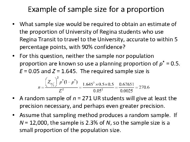
Example of sample size for a proportion • What sample size would be required to obtain an estimate of the proportion of University of Regina students who use Regina Transit to travel to the University, accurate to within 5 percentage points, with 90% confidence? • For this question, neither the sample nor population proportion are known so use a planning proportion of p* = 0. 5. E = 0. 05 and Z = 1. 645. The required sample size is • A random sample of n = 271 UR students will give at least the precision necessary, and perhaps even greater precision. • Assume that sampling method produces a random sample. If N = 12, 000, the sample is 2. 3% of N, so the sample size is a small proportion of the population size.

Notes about sample size for estimating a population proportion • Random sample of a population. • If the sample size is a small proportion of the population size (less than 5 -10% of population), then it does not matter how large the population is, the required n is independent of population size. • This formula is especially useful, since it does not require knowledge of the population variability. If p* = 0. 5 is used in the above formula, the sample size will be more than sufficient to achieve the required margin of error with the specified level of confidence. • Not too many nonsampling errors such as poorly constructed questions, nonresponse, refusals, etc. • For more complex sampling procedures, consult a text on sampling procedures.

• Monday, Oct. 20 – we will discuss the above slides and then have some time for review. • Tuesday, Oct. 21, 3: 30 – 4: 30 p. m. Optional review period with your two instructors. CL 232. • Wednesday, Oct. 22, 2: 30 – 3: 45 is the midterm. You are permitted to bring a text, photocopies of the tables (normal, t, binomial), and one extra sheet. Make sure you bring a calculator. No communication with other individuals inside or outside of the classroom using electronic devices. • The midterm covers the topics discussed in class to October 20, that is, the assigned sections of chapters 1 -8 of the text and any additional materials discussed in class. • We are hoping to have Assignment 3 graded and available to pick up at the Tuesday review session. Answers will be posted on UR Courses some time on Tuesday.