Chapter 7 Estimating Parameters and Determining Sample Sizes

Chapter 7 Estimating Parameters and Determining Sample Sizes Presented by: Nada Alzahrani Atheer Bin Safiran Jumana Alsanousi

7 -1 Estimating a Population Proportion 7 -2 Estimating a Population Mean 7 -3 Estimating a Population Standard Deviation or Variance

Chapter 7 In this chapter we begin the study of methods of inferential statistics. Major Activities of Inferential Statistics: 1 -Use sample data to estimate values of population parameters. 2 -Use sample data to test hypotheses made about population parameters.

Estimating a Population Proportion Key Concept In this section we present methods for using a sample proportion to estimate the value of a population proportion.

Three main concepts – Point Estimate: The sample proportion is the best point estimate of the population proportion. – Confidence Interval: We can use a sample proportion to construct a confidence interval estimate of the true value of a population proportion, and we should know how to interpret such confidence intervals. – Sample Size: We should know how to find the sample size necessary to estimate a population proportion.

Point Estimate Definition: A point estimate is a single value used to estimate a population parameter. – The sample proportion pˆ is the best point estimate of the population proportion p.

Notation – p population proportion. Note: proportion, percentage, and probability can all be considered as p. – pˆ sample proportion

Example: The Pew Research Center conducted a survey of 1007 adults and found that 85% of them know what twitter is. The best point estimate of p, the population proportion, is the sample proportion: pˆ= 0. 85

Confident Interval Definition A confidence interval (or interval estimate) is a range (or an interval) of values used to estimate the true value of a population parameter. A confidence interval is sometimes abbreviated as CI.

Confidence level Is the probability 1 -α that the confidence interval contains the true population parameter that is being estimated, assuming that the estimation process is repeated a large number of times. (the confidence level is also called the degree of confidence, or the confidence coefficient.

Confidence level The following table shows the relationship between the confidence level and the corresponding values of α Most Common Confidence Levels Corresponding Values of α 90% (or 0. 90) confidence level α= 0. 10 95% (or 0. 95) confidence level α= 0. 05 99% (or 0. 99) confidence level α= 0. 01

Interpreting a Confidence Interval We must be careful to interpret confidence intervals correctly. There is a correct interpretation and many different incorrect interpretations of confidence interval 0. 828< p < 0. 872 “We are 95% confident that the interval from 0. 828 to 0. 872 actually does contain the true value of the population proportion p. ” This means that if we were to select many different samples of size 1007 and construct the corresponding confidence intervals, 95% of them would actually contain the value of the population proportion p.

Critical Values A standard z score can be used to distinguish between sample statistics that are likely to occur and those that are unlikely to occur. Such a z score is called a critical value. Critical values are based on the following observations: 1 -Under certain conditions, the sampling distribution of sample proportions can be approximated by a normal distribution.

2 -A z score associated with a sample proportion has a probability of /2 of falling in the right tail portion. 3 - The z score at the boundary of the right-tail region is commonly denoted by z /2 and is referred to as a critical value because it is on the borderline separating z scores that are significantly high.

Definition A critical value is the number on the borderline separating sample statistics that are likely to occur from those that are unlikely to occur. The number z /2 is a critical value that is a z score with the property that it separates an area of /2 in the right tail of the standard normal distribution.

The Critical Value z 2

z 2 for a 95% Confidence Level

Common Critical Values Confidence Level Critical Value, z /2 90% 0. 10 1. 645 95% 0. 05 1. 96 99% 0. 01 2. 575

Margin of Error When data from a simple random sample are used to estimate a population proportion p, the margin of error, denoted by E, is the maximum likely difference (with probability 1 – , such as 0. 95) between the observed proportion and the true value of the population proportion p. The margin of error E is also called the maximum error of the estimate and can be found by multiplying the critical value and the standard deviation of the sample proportions.

Margin of Error for Proportions

Confidence Interval for Estimating a Population Proportion p – p = population proportion – pˆ= sample proportion – n = number of sample values – E = margin of error – z /2 = z score separating an area of /2 in the right tail of the standard normal distribution

Requirements for Using a Confidence Interval for Estimating a Population Proportion p 1. The sample is a simple random sample. 2. The conditions for the binomial distribution are satisfied: there is a fixed number of trials, the trials are independent, there are two categories of outcomes, and the probabilities remain constant for each trial. 3. There at least 5 successes and 5 failures.

Confidence Interval for Estimating a Population Proportion p pˆ– E < pˆ + E Where:

The confidence interval is often expressed in the following format: Pˆ+-E or (pˆ– E, pˆ + E)

Procedure for Constructing a Confidence Interval for p 1 -Verify that the required assumptions are satisfied. 2 -Refer to Table A-2 and find the critical value z��/2 that corresponds to the desired confidence level. 3. Evaluate the margin of error

4. Using the value of the calculated margin of error, E and the value of the sample proportion, pˆ, find the values of pˆ – E and pˆ+ E. Substitute those values in the general format for the confidence interval: pˆ– E < pˆ + E 5. Round digits. the resulting confidence interval limits to three significant

Example The Pew Research Center conducted a survey of 1007 randomly selected adults and found that 85% of them know what twitter is. The sample results are n=1007 and pˆ=0. 70 1 - Find the margin of error E that corresponds to a 95% confidence level. 2 - Find the 95% confidence interval estimate of the population proportion p 3 - Based on the results can we safely conclude that more than 75% of adults know what twitter is?

Example Margin of error E 1. 96 √(0. 85)(0. 15) / 1007 E= 0. 0220545

2 - The 95% confidence interval pˆ– E < pˆ + E 0. 85 - 0. 0220545 < p < 0. 85+ 0. 0220545 0. 828 < p < 0. 872

3 -Based on the results can we safely conclude that more than 75% of adults know what twitter is? Based on the confidence interval, it does appear that more than 75% of adults know what twitter is. Because the limits of 0. 828 and 0. 872 are likely to contain the true population proportion, it appears that population proportion is value greater than 0. 75.

Finding the Point Estimate and E from a Confidence Interval If we already know the confidence interval limits, the sample proportion (or the best point estimate) pˆ and the margin of error E can be found as the following:

Example: The article “High-Dose Nicotine Patch Therapy”, includes this statement: “ of the 71 subjects, 70% were abstinent from smoking at 8 weeks (95% confidence interval CI, 58% to 81%). Find the point estimate pˆ and the margin error E

Sample Size Suppose we want to collect sample data in order to estimate some population proportion. The question is how many sample items must be obtained?

Determining Sample Size When an estimate of pˆ is known

When no estimate of pˆ is known:

Example If we were to conduct a survey to determine the percentage of children (older than 1 year) who have received measles vaccinations, how many children must be surveyed in order to be 95% confident that the sample percentage is in error by no more than three percentage points? a- Assume that a recent survey showed that 90% of children have received measles vaccinations. b- Assume that we have no prior information suggesting a possible value of the population proportion.

a. With a 95% confidence level, we have =0. 05, so z /2 = 1. 96. Also, the margin of error is E=0. 03, which is the decimal equivalent of three percentage points. pˆ=0. 90, so qˆ =0. 10. Because we have an estimated value of pˆ we use this formula

Example b. With no prior knowledge of pˆ (or qˆ ) we use:

Estimating a Population Mean: Not Known (common) Atheer Bin Safiran

Key Concept – This section presents methods for estimating a population mean when the population standard deviation is not known. With σ unknown, we use the Student t distribution assuming that the relevant requirements are satisfied.

Point Estimate – The Sample Mean is the best point estimate of the population mean.

Notation = population mean = sample mean s = sample standard deviation n = number of sample values E = margin of error

Requirement of “Normality or n >30” – Normality: The normality requirement is loose. The distribution need not be perfectly bell-shaped, but it should appear to be somewhat symmetric with one mode and no outliers. – Sample size n > 30 : sample sizes of 15 to 30 are adequate if the population appears to have a distribution that is no far from being normal and there are no outliers.

Student t Distribution – If the distribution of a population is essentially normal, then the distribution of t = x-µ s n is a Student t Distribution for all samples of size n. It is often referred to as a t distribution and is used to find critical values denoted by t /2.

Important Properties of the Student t Distribution Ø The Student t distribution has the same general symmetric bell shape as the standard normal distribution but has more variability (with wider distributions) as we expected with small samples. Ø The Student t distribution has a mean of t = 0 (just as the standard normal distribution has a mean of z = 0). Ø The standard deviation of the Student t distribution varies with the sample size and is greater than 1 (unlike the standard normal distribution, which has a = 1). Ø The Student t distribution is different for different sample sizes (see the following slide, for the cases n = 3 and n = 12). As the sample size n gets larger, the Student t distribution gets closer to the normal distribution.

Student t Distributions for n = 3 and n = 12

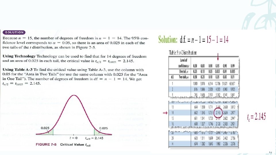
Definition : Degrees of Freedom – The number of degrees of freedom for a collection of sample data is the number of sample values that can vary after certain restrictions have been imposed on all data values. The degree of freedom is often abbreviated df. Degrees of freedom = n – 1

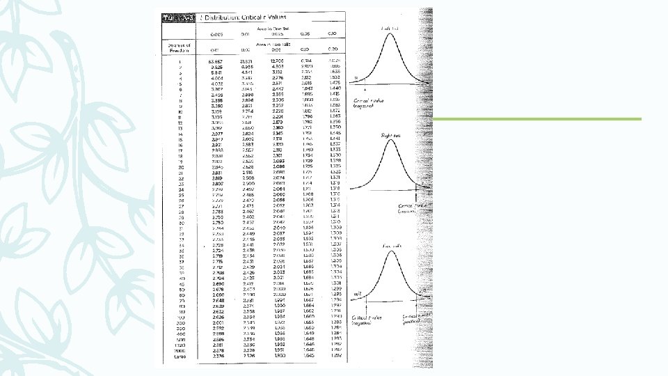
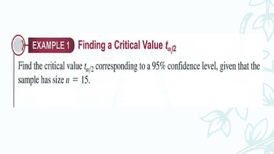
How to Find a T Critical Value t 2 – A critical value t 2 can be found using table A-3 with selected numbers of degree of freedom. Table A-3 lists values for tα/2

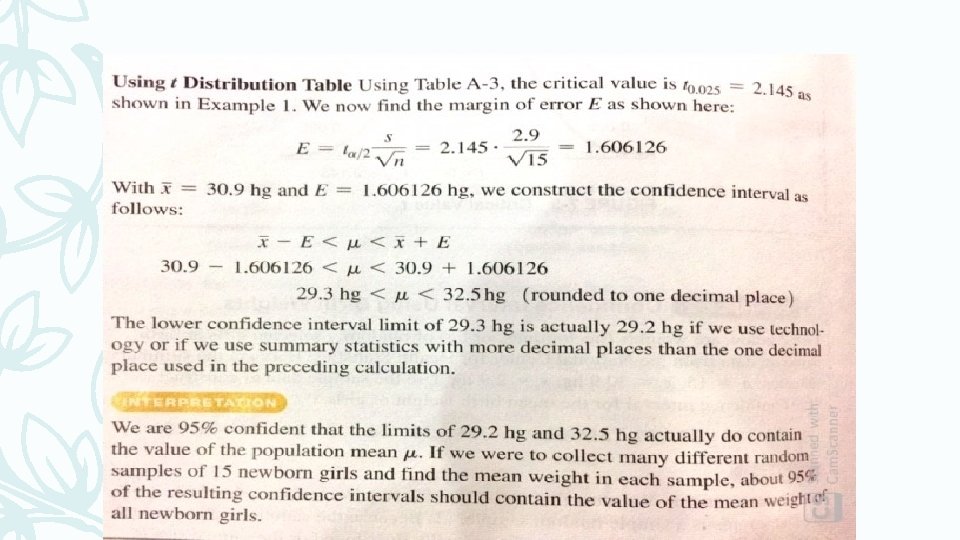
Margin of Error E for Estimate of (With σ Not Known) E = t / s 2 n where t 2 has n – 1 degrees of freedom.

Confidence Interval for the Estimate of μ (With σ Not Known) x–E <µ<x +E where E = t /2 s n df = n – 1 t /2 found in Table A-3

Requirements for Using a Confidence Interval for Estimating a Population Mean µ 1. The sample is a simple random sample. 2. Either the sample is from a normally distributed population or n>30

Procedure for Constructing a Confidence Interval for µ (With σ Unknown) 1. Verify that the requirements are satisfied. 2. Using n – 1 degrees of freedom, refer to Table A-3 or use technology to find the critical value t 2 that corresponds to the desired confidence level. 3. Evaluate the margin of error E = t 2 • s / n. 4. Find the values of Substitute those values in the general format for the confidence interval: 5. Round the resulting confidence interval limits.

Example: Construct the confidence interval estimate of the mean

Example – Use the sample statistics of – n = 49, = 0. 4 and s = 21. 0 – to construct a 95% confidence interval estimate of the population mean.

Example – 95% confidence level so – = 5%=0. 05 With n = 49, the df = 49 – 1 = 48 Closest df in Table A-3 is 50, using two tails = 5%=0. 05 using one tail /2= 2. 5%=0. 025 t /2 = 2. 009

Using t /2 = 2. 009, s = 21. 0 and n = 49 the margin of error is: and the confidence interval is

Finding the Point Estimate and E from a Confidence Interval Point estimate of µ: x = (upper confidence limit) + (lower confidence limit) 2 Margin of Error: E = (upper confidence limit) - (lower confidence limit) 2

Example: The confidence interval (10. 0, 30. 0) yields x = (upper confidence limit) + (lower confidence limit) 2 X = 30. 0+ 10. 0 = 20. 0 2 E = (upper confidence limit) - (lower confidence limit) 2 E = 30. 0 – 10. 0 = 10. 0 2

Estimating a Population Mean: σ Known (rare) – It is extremely rare that we want to estimate the population mean µ but we somehow know the value of the population standard deviation σ. – The confidence interval is constructed using the standard normal distribution instead of the Student t distribution. – Margin of error used with known σ

Example:

Solution:

Choosing the Appropriate Distribution:

Thank you