ROOT Graphics Status and Future Plans Olivier Couet

ROOT Graphics: Status and Future Plans Olivier Couet (CERN) CHEP 2007 2 -7 September 2007

Overview • • Basic Elements of ROOT Graphics. 2 D Graphics Latest Developments. 3 D Graphics Latest Developments. Multiple Variable Data Set Visualization. • Spider (Radar) Plots. • Parallel Coordinates Plots. • Box (Candle) Plots. • Conclusion. Olivier Couet CHEP 2007 2 -7 September 2007 2

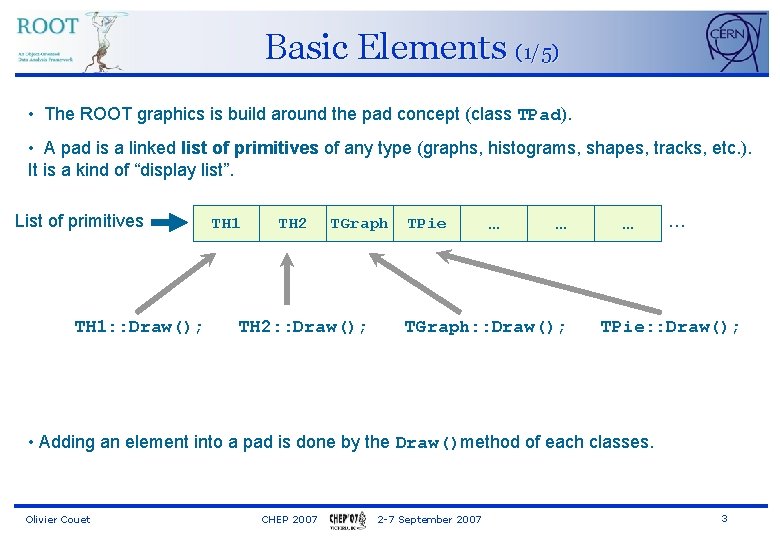
Basic Elements (1/5) • The ROOT graphics is build around the pad concept (class TPad). • A pad is a linked list of primitives of any type (graphs, histograms, shapes, tracks, etc. ). It is a kind of “display list”. List of primitives TH 1: : Draw(); TH 1 TH 2 TGraph TH 2: : Draw(); TPie … … TGraph: : Draw(); … … TPie: : Draw(); • Adding an element into a pad is done by the Draw()method of each classes. Olivier Couet CHEP 2007 2 -7 September 2007 3

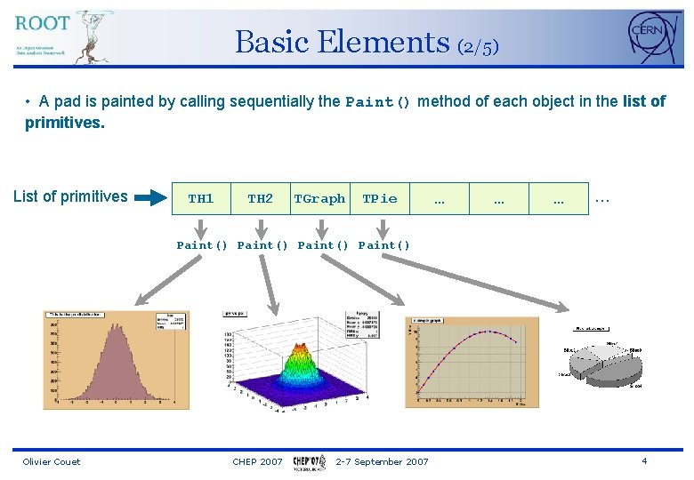
Basic Elements (2/5) • A pad is painted by calling sequentially the Paint() method of each object in the list of primitives. List of primitives TH 1 TH 2 TGraph TPie … … Paint() Olivier Couet CHEP 2007 2 -7 September 2007 4

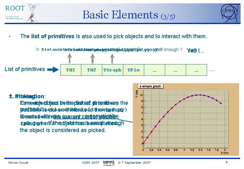
Basic Elements (3/5) • The list of primitives is also used to pick objects and to interact with them. Is Distanceto. Primitive(px, py)small enough ? Is Distanceto. Primitive(px, py)small List of primitives TH 1 TH 2 TGraph TPie … … Yes NO !… … … 1. 2. Picking: Interaction: For Oneeach object has been in thepicked. list of primitives It is now the method possible. Distanceto. Primitive(px, py) to act on it thanks to the method Execute. Event(px, py)automatically is called with the current cursor position (px, py). theobject distance small enough called when. Ifan hasisbeen picked. the object is considered as picked. Olivier Couet CHEP 2007 2 -7 September 2007 5

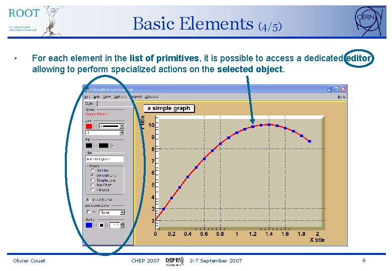
Basic Elements (4/5) • For each element in the list of primitives, it is possible to access a dedicated editor allowing to perform specialized actions on the selected object. Olivier Couet CHEP 2007 2 -7 September 2007 6

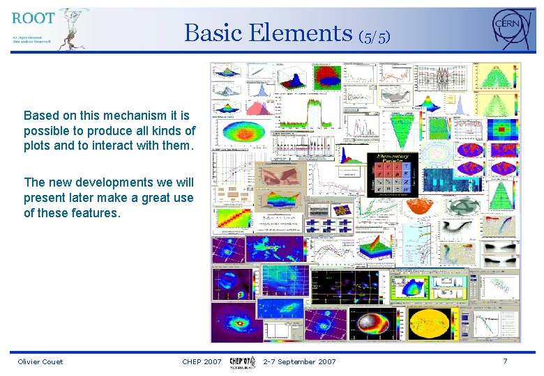
Basic Elements (5/5) Based on this mechanism it is possible to produce all kinds of plots and to interact with them. The new developments we will present later make a great use of these features. Olivier Couet CHEP 2007 2 -7 September 2007 7

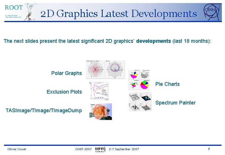
2 D Graphics Latest Developments The next slides present the latest significant 2 D graphics’ developments (last 18 months): Polar Graphs Pie Charts Exclusion Plots Spectrum Painter TASImage/TImage. Dump Olivier Couet CHEP 2007 2 -7 September 2007 8

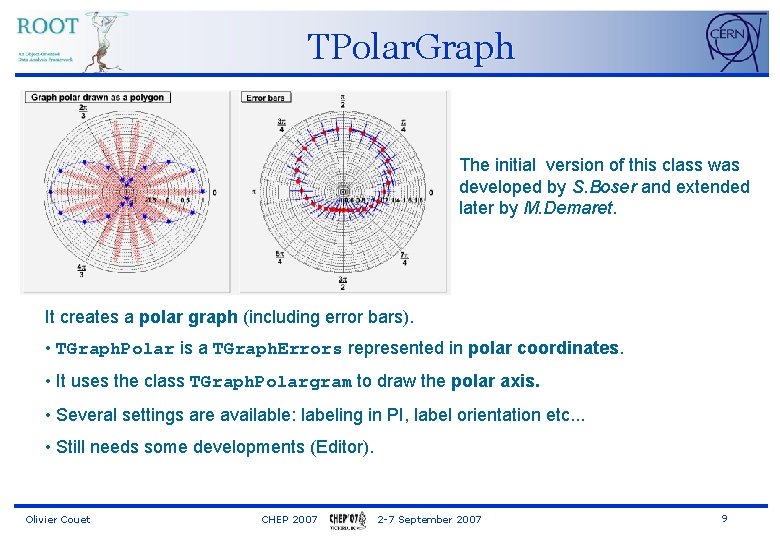
TPolar. Graph The initial version of this class was developed by S. Boser and extended later by M. Demaret. It creates a polar graph (including error bars). • TGraph. Polar is a TGraph. Errors represented in polar coordinates. • It uses the class TGraph. Polargram to draw the polar axis. • Several settings are available: labeling in PI, label orientation etc. . . • Still needs some developments (Editor). Olivier Couet CHEP 2007 2 -7 September 2007 9

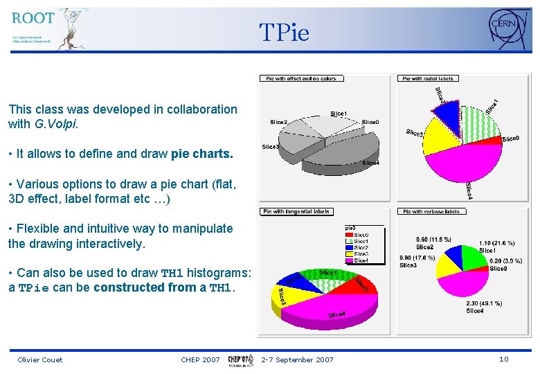
TPie This class was developed in collaboration with G. Volpi. • It allows to define and draw pie charts. • Various options to draw a pie chart (flat, 3 D effect, label format etc …) • Flexible and intuitive way to manipulate the drawing interactively. • Can also be used to draw TH 1 histograms: a TPie can be constructed from a TH 1. Olivier Couet CHEP 2007 2 -7 September 2007 10

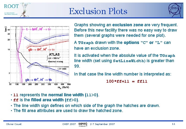
Exclusion Plots Graphs showing an exclusion zone are very frequent. Before this new facility there was no easy way to draw them (several graphs were needed for one plot). A TGraph drawn with the options "C" or "L" can have an exclusion zone. It is activated when the absolute value of the TGraph line width (set using Set. Line. Width) is greater than 99. In that case the line width number is interpreted as: 100*ff+ll = ffll • ll represents the normal line width (ll>0). • ff is the filled area width (ff>0). • The line width sign defines on which side of the graph the hatches are drawn. • The fill area attributes are used to draw the hatched zone. Olivier Couet CHEP 2007 2 -7 September 2007 11

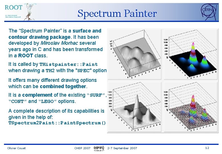
Spectrum Painter The “Spectrum Painter” is a surface and contour drawing package. It has been developed by Miroslav Morhac several years ago in C and has been transformed in a ROOT class. It is called by THistpainter: : Paint when drawing a TH 2 with the "SPEC" option. It offers many different drawing options which can be combined together. It is a complement of the existing “SURF”, “CONT” and “LEGO” options. A complete description of its capabilities is given in the help of: TSpectrum 2 Paint: : Paint. Spectrum() Olivier Couet CHEP 2007 2 -7 September 2007 12

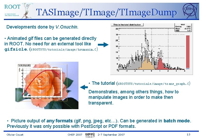
TASImage/TImage. Dump Developments done by V. Onuchin. • Animated gif files can be generated directly in ROOT. No need for an external tool like gifsicle. ($ROOTSYS/tutorials/image/ hsumanim. C) • The tutorial ($ROOTSYS/tutorials/image/ trans_graph. C ) Demonstrates, among others things, how to manipulate images in order to make then transparent. • Picture output of any formats (gif, png, jpeg, etc…). Can be generated in batch mode. Previously it was only possible with Post. Script or PDF formats. Olivier Couet CHEP 2007 2 -7 September 2007 13

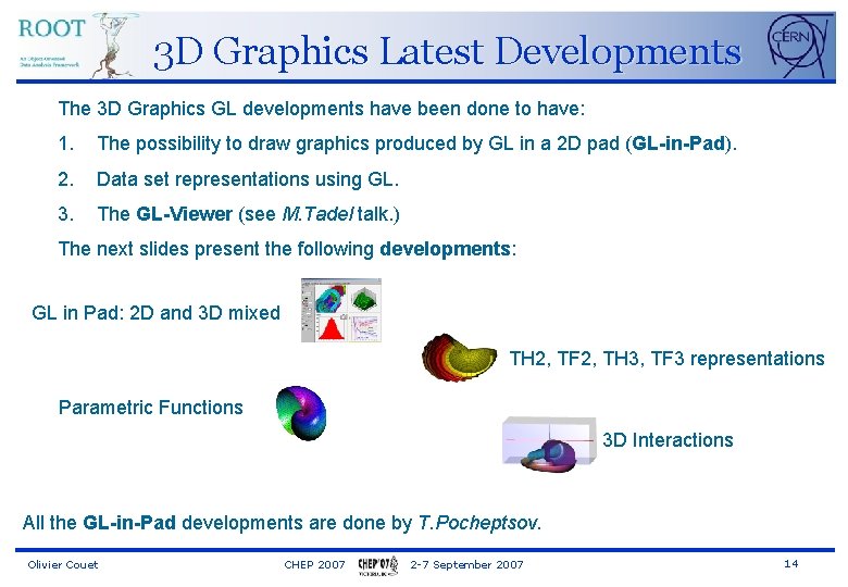
3 D Graphics Latest Developments The 3 D Graphics GL developments have been done to have: 1. The possibility to draw graphics produced by GL in a 2 D pad (GL-in-Pad). 2. Data set representations using GL. 3. The GL-Viewer (see M. Tadel talk. ) The next slides present the following developments: GL in Pad: 2 D and 3 D mixed TH 2, TF 2, TH 3, TF 3 representations Parametric Functions 3 D Interactions All the GL-in-Pad developments are done by T. Pocheptsov. Olivier Couet CHEP 2007 2 -7 September 2007 14

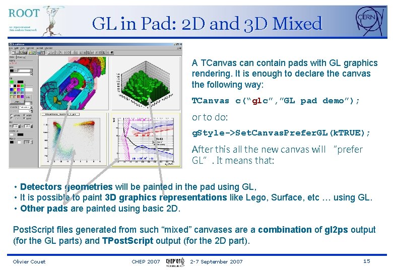
GL in Pad: 2 D and 3 D Mixed A TCanvas can contain pads with GL graphics rendering. It is enough to declare the canvas the following way: TCanvas c(“glc”, ”GL pad demo”); or to do: g. Style->Set. Canvas. Prefer. GL(k. TRUE); After this all the new canvas will “prefer GL”. It means that: • Detectors geometries will be painted in the pad using GL, • It is possible to paint 3 D graphics representations like Lego, Surface, etc … using GL. • Other pads are painted using basic 2 D. Post. Script files generated from such “mixed” canvases are a combination of gl 2 ps output (for the GL parts) and TPost. Script output (for the 2 D part). Olivier Couet CHEP 2007 2 -7 September 2007 15

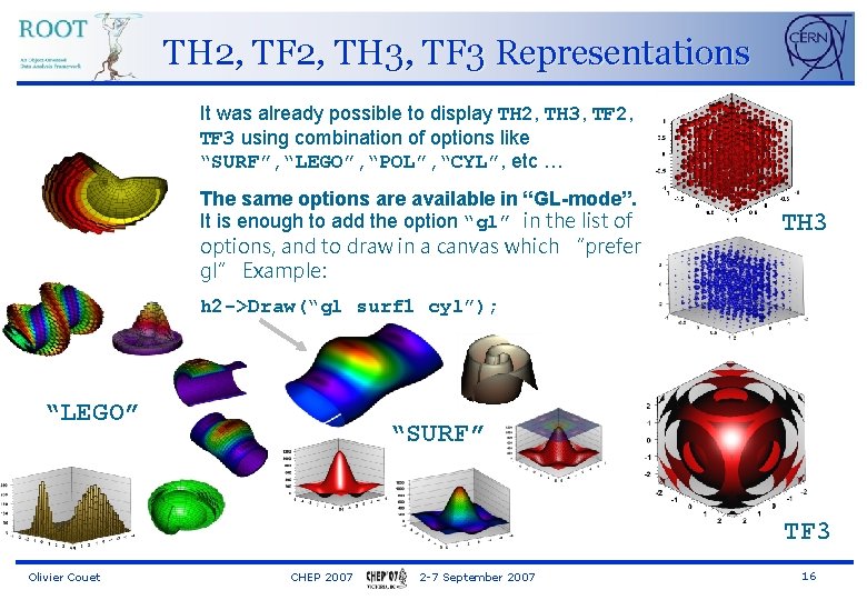
TH 2, TF 2, TH 3, TF 3 Representations It was already possible to display TH 2, TH 3, TF 2, TF 3 using combination of options like “SURF”, “LEGO”, “POL”, “CYL”, etc … The same options are available in “GL-mode”. It is enough to add the option “gl” in the list of options, and to draw in a canvas which “prefer gl” Example: TH 3 h 2 ->Draw(“gl surf 1 cyl”); “LEGO” “SURF” TF 3 Olivier Couet CHEP 2007 2 -7 September 2007 16

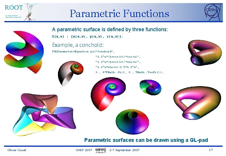
Parametric Functions A parametric surface is defined by three functions: S(u, v) : {x(u, v), y(u, v), z(u, v)}. Example, a conchoid: TGLParametric. Equation p 1("Conchoid", "1. 2^u*(1+cos(v))*cos(u)", "1. 2^u*(1+cos(v))*sin(u)", "1. 2^u*sin(v)-1. 5*1. 2^u", 0. , 6*TMath: : Pi(), 0. , TMath: : Two. Pi()); Parametric surfaces can be drawn using a GL-pad Olivier Couet CHEP 2007 2 -7 September 2007 17

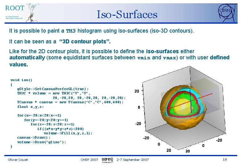
Iso-Surfaces It is possible to paint a TH 3 histogram using iso-surfaces (iso-3 D contours). It can be seen as a “ 3 D contour plots”. Like for the 2 D contour plots, it is possible to define the iso-surfaces either automatically (some equidistant surfaces between vmin and vmax) or with user defined values. void iso() { g. Style->Set. Canvas. Prefer. GL(true); TH 3 C * volume = new TH 3 C("V", 20, -20, 20, 20, -20, 20); TCanvas * canvas = new TCanvas("C", 600, 600); float x, y, z; for(x=-20; x<20; x+=1) for(y=-20; y<20; y+=1) for(z=-20; z<20; z+=1) if((x*x+y*y+z*z)<200) volume->Fill(x, y, z, 1); canvas->Draw(); volume->Draw("gliso"); } Olivier Couet CHEP 2007 2 -7 September 2007 18

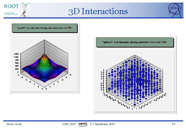
3 D Interactions Olivier Couet CHEP 2007 2 -7 September 2007 19

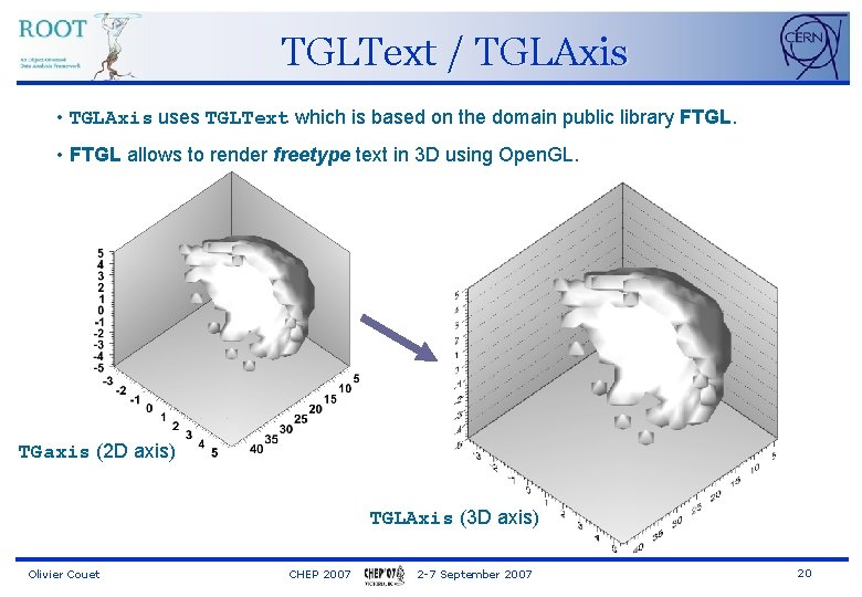
TGLText / TGLAxis • TGLAxis uses TGLText which is based on the domain public library FTGL. • FTGL allows to render freetype text in 3 D using Open. GL. TGaxis (2 D axis) TGLAxis (3 D axis) Olivier Couet CHEP 2007 2 -7 September 2007 20

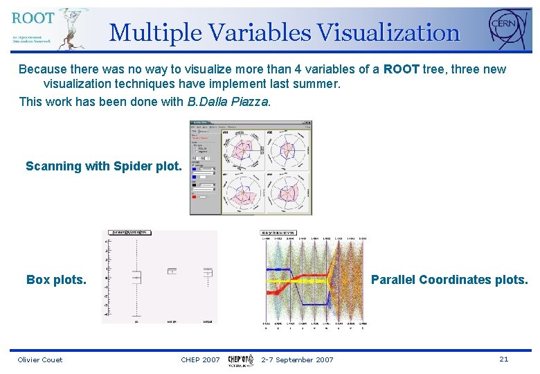
Multiple Variables Visualization Because there was no way to visualize more than 4 variables of a ROOT tree, three new visualization techniques have implement last summer. This work has been done with B. Dalla Piazza. Scanning with Spider plot. Box plots. Olivier Couet Parallel Coordinates plots. CHEP 2007 2 -7 September 2007 21

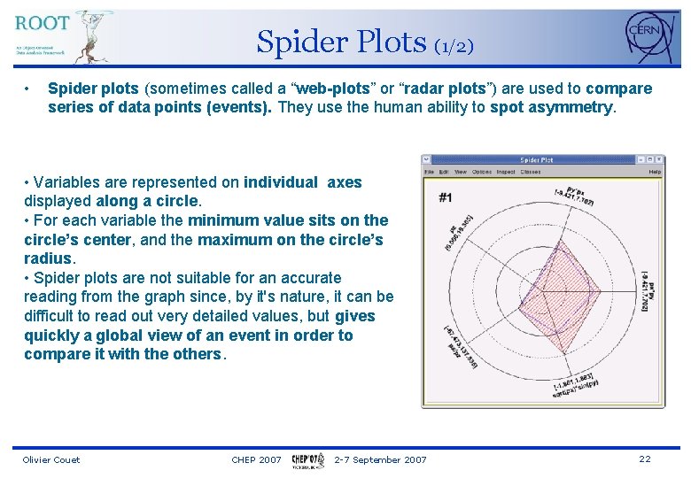
Spider Plots (1/2) • Spider plots (sometimes called a “web-plots” or “radar plots”) are used to compare series of data points (events). They use the human ability to spot asymmetry. • Variables are represented on individual axes displayed along a circle. • For each variable the minimum value sits on the circle’s center, and the maximum on the circle’s radius. • Spider plots are not suitable for an accurate reading from the graph since, by it's nature, it can be difficult to read out very detailed values, but gives quickly a global view of an event in order to compare it with the others. Olivier Couet CHEP 2007 2 -7 September 2007 22

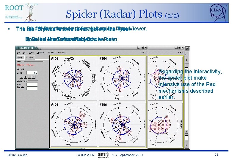
Spider (Radar) Plots (2/2) • The Spider tab “Style” Plotallows can betoaccessed define thefrom spider Tree “Browse” allows to navigate in the layout. Tree. Viewer. 2) Select the Spider Plot view Note 1) the other Tree of drawing variables Spider to be. Plots. seen. Regarding the interactivity, the spider plot make intensive use of the Pad mechanisms described earlier. Olivier Couet CHEP 2007 2 -7 September 2007 23

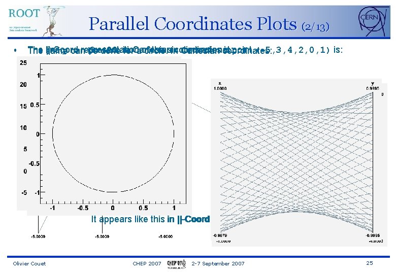
Parallel Coordinates Plots (1/13) • The multidimensional system of Parallel Coordinates Plots (||-Coord) is a common way of studying and visualizing multivariate data sets. They were proposed by in A. Inselberg in 1981 as a new way to represent multidimensional information. • In traditional Cartesian coordinates, axes are mutually perpendicular. In Parallel coordinates, all axes are parallel which allows to represent data in much more than 3 dimensions. • A point in n-dimensional space is represented as a polyline with vertices on the parallel axes. The position of the vertex on the i-th axis corresponds to the i-th coordinate of the point. • To show a set of points in ||-Coord, a set of parallel lines is drawn, typically vertical and equally spaced. Olivier Couet CHEP 2007 2 -7 September 2007 24

Parallel Coordinates Plots (2/13) • The ||-Coord line y can = representation -3 x+20 the six dimensional is: point (-5, 3, 4, 2, 0, 1) is: same be done in for. Cartesian aof circle. Incoordinates Cartesian coordinates: It appears like this in ||-Coord: Olivier Couet CHEP 2007 2 -7 September 2007 25

Parallel Coordinates Plots (3/13) • ||-Coord plots are a widely used technique to display and explore multi-dimensional data. • It is good at: spotting irregular events, see the data trend, finding correlations and clusters. • Its main weakness: the cluttering of the output. But there are techniques to bypass it. This summer, we have implemented ||-Coord plots in ROOT as a new plotting option “PARA” in the TTree: : Draw() method. Olivier Couet CHEP 2007 2 -7 September 2007 26

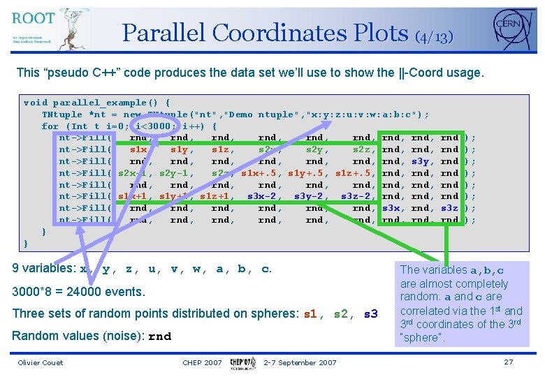
Parallel Coordinates Plots (4/13) This “pseudo C++” code produces the data set we’ll use to show the ||-Coord usage. void parallel_example() { TNtuple *nt = new TNtuple("nt", "Demo ntuple", "x: y: z: u: v: w: a: b: c"); for (Int_t i=0; i<3000; i++) { nt->Fill( rnd, rnd, nt->Fill( s 1 x, s 1 y, s 1 z, s 2 x, s 2 y, s 2 z, rnd, nt->Fill( rnd, rnd, s 3 y, nt->Fill( s 2 x-1, s 2 y-1, s 2 z, s 1 x+. 5, s 1 y+. 5, s 1 z+. 5, rnd, nt->Fill( rnd, rnd, nt->Fill( s 1 x+1, s 1 y+1, s 1 z+1, s 3 x-2, s 3 y-2, s 3 z-2, rnd, nt->Fill( rnd, rnd, s 3 x, rnd, nt->Fill( rnd, rnd, } } 9 variables: x, y, z, u, v, w, a, b, c. 3000*8 = 24000 events. Three sets of random points distributed on spheres: s 1, s 2, s 3 Random values (noise): rnd Olivier Couet CHEP 2007 2 -7 September 2007 rnd rnd rnd s 3 z rnd ); ); The variables a, b, c 2 6 “spheres” correlated are by 2 almost on thecompletely variables random. a and x, y, z, u, v, w c are correlated via the 1 st and 3 rd coordinates of the 3 rd “sphere”. 27

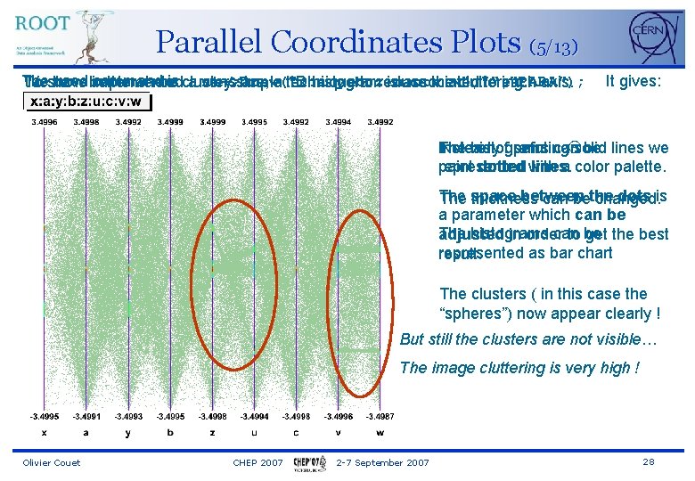
Parallel Coordinates Plots (5/13) The used better command is: clusters nt->Draw("x: a: y: b: z: u: c: v: w", "PARA"); To show We have implemented where a very simple are, a technique 1 D histogram to reduce is associated the cluttering. to each axis. It gives: Instead The histograms ofuseful painting cansolid be lines we Not very … represented paint dotted with lines. a color palette. The space between dots is thickness can bethe changed. a parameter which can be The histograms can adjusted in order to be get the best represented as bar chart result. The clusters ( in this case the “spheres”) now appear clearly ! But still the clusters are not visible… The image cluttering is very high ! Olivier Couet CHEP 2007 2 -7 September 2007 28

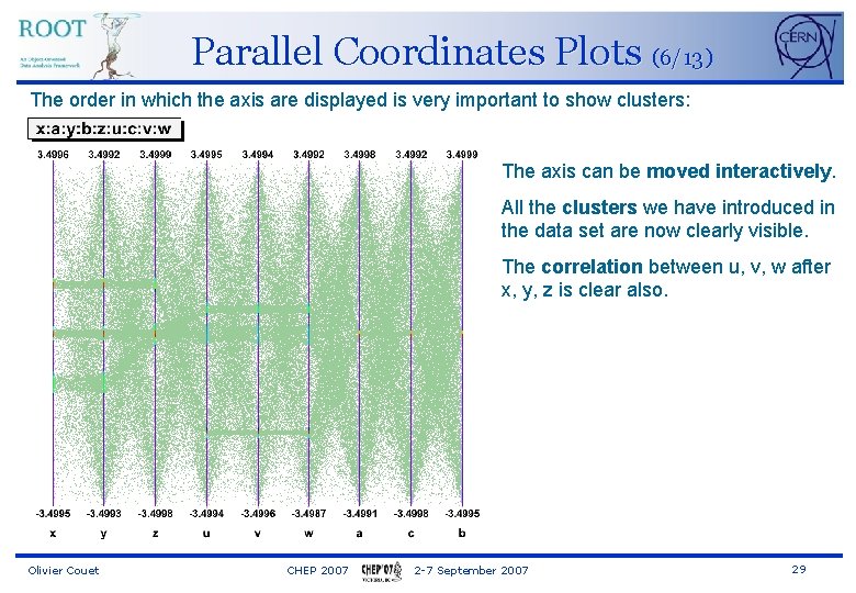
Parallel Coordinates Plots (6/13) The order in which the axis are displayed is very important to show clusters: The axis can be moved interactively. All the clusters we have introduced in the data set are now clearly visible. The correlation between u, v, w after x, y, z is clear also. Olivier Couet CHEP 2007 2 -7 September 2007 29

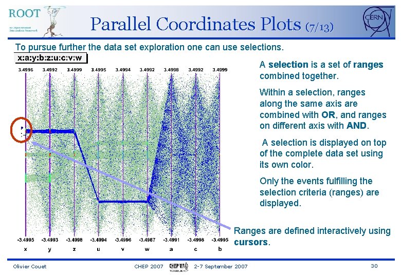
Parallel Coordinates Plots (7/13) To pursue further the data set exploration one can use selections. A selection is a set of ranges combined together. Within a selection, ranges along the same axis are combined with OR, and ranges on different axis with AND. A selection is displayed on top of the complete data set using its own color. Only the events fulfilling the selection criteria (ranges) are displayed. Ranges are defined interactively using cursors. Olivier Couet CHEP 2007 2 -7 September 2007 30

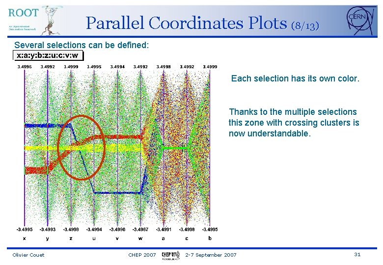
Parallel Coordinates Plots (8/13) Several selections can be defined: Each selection has its own color. Thanks to the multiple selections this zone with crossing clusters is now understandable. Olivier Couet CHEP 2007 2 -7 September 2007 31

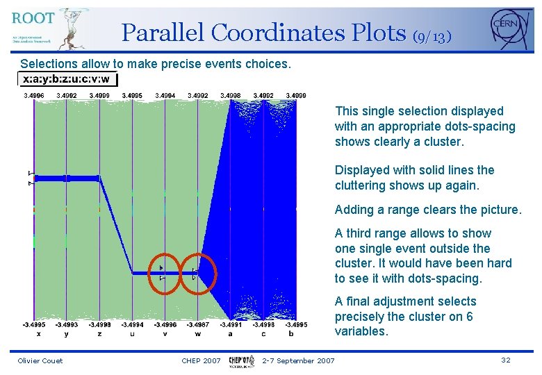
Parallel Coordinates Plots (9/13) Selections allow to make precise events choices. This single selection displayed with an appropriate dots-spacing shows clearly a cluster. Displayed with solid lines the cluttering shows up again. Adding a range clears the picture. A third range allows to show one single event outside the cluster. It would have been hard to see it with dots-spacing. A final adjustment selects precisely the cluster on 6 variables. Olivier Couet CHEP 2007 2 -7 September 2007 32

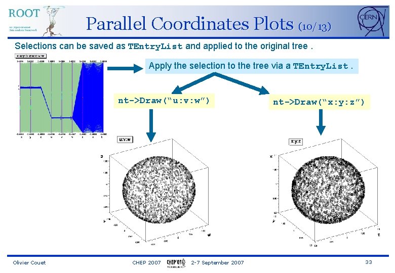
Parallel Coordinates Plots (10/13) Selections can be saved as TEntry. List and applied to the original tree. Apply the selection to the tree via a TEntry. List. nt->Draw(“u: v: w”) Olivier Couet CHEP 2007 2 -7 September 2007 nt->Draw(“x: y: z”) 33

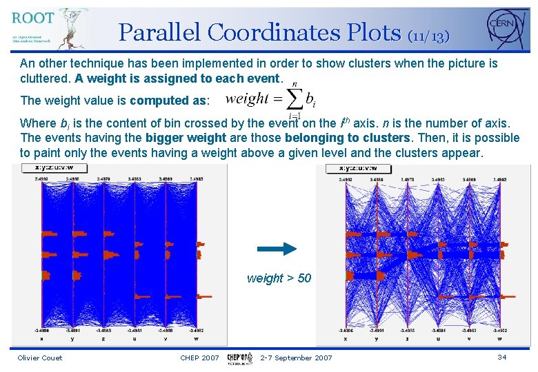
Parallel Coordinates Plots (11/13) An other technique has been implemented in order to show clusters when the picture is cluttered. A weight is assigned to each event. The weight value is computed as: Where bi is the content of bin crossed by the event on the ith axis. n is the number of axis. The events having the bigger weight are those belonging to clusters. Then, it is possible to paint only the events having a weight above a given level and the clusters appear. weight > 50 Olivier Couet CHEP 2007 2 -7 September 2007 34

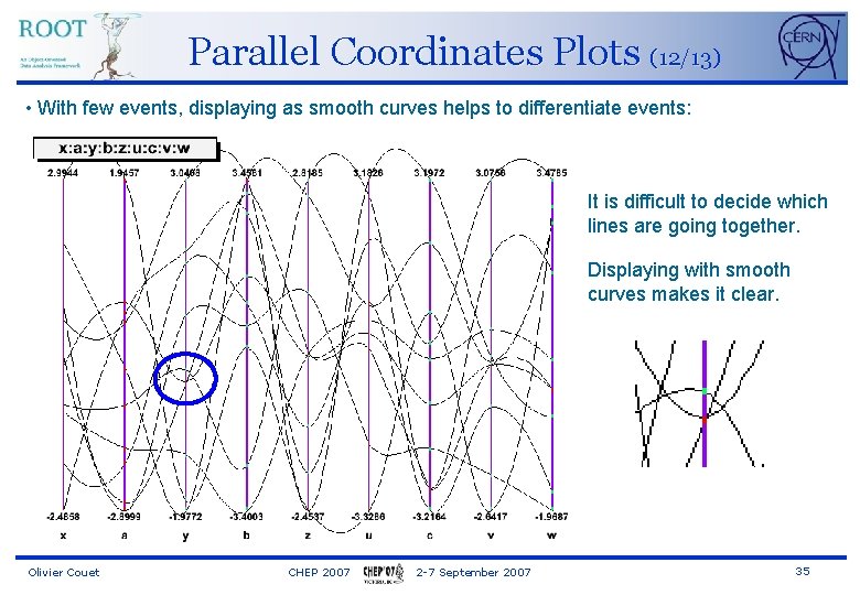
Parallel Coordinates Plots (12/13) • With few events, displaying as smooth curves helps to differentiate events: It is difficult to decide which lines are going together. Displaying with smooth curves makes it clear. Olivier Couet CHEP 2007 2 -7 September 2007 35

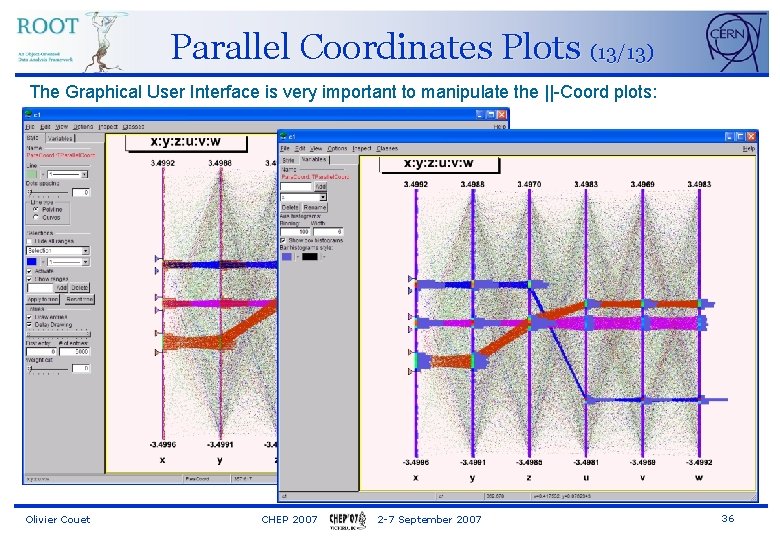
Parallel Coordinates Plots (13/13) The Graphical User Interface is very important to manipulate the ||-Coord plots: Olivier Couet CHEP 2007 2 -7 September 2007 36

Box Plots (1/3) • A Box Plot (also known as a “box-and whisker” plot or “candle stick” plot) is a convenient way to describe graphically a data distribution (D) with only the five numbers. It was invented in 1977 by John Tukey. • The five numbers are: 1. The minimum value of the distribution D (Min). 2. The lower quartile (Q 1): 25% of the data points in D are less than Q 1. 3. The median (M): 50% of the data points in D are less than M. 4. The upper quartile (Q 3): 75% of the data points in D are less than Q 3. 5. The maximum value of the distribution D (Max). Olivier Couet CHEP 2007 2 -7 September 2007 37

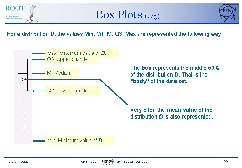
Box Plots (2/3) For a distribution D, the values Min, Q 1, M, Q 3, Max are represented the following way: Maximum value of D. Q 3: Upper quartile. The box represents the middle 50% of the distribution D. That is the "body" of the data set. M: Median. Q 2: Lower quartile. Very often the mean value of the distribution D is also represented. Min: Minimum value of D. Olivier Couet CHEP 2007 2 -7 September 2007 38

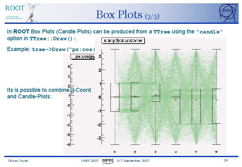
Box Plots (3/3) In ROOT Box Plots (Candle Plots) can be produced from a TTree using the “candle” option in TTree: : Draw(): Example: tree->Draw(“px: cos(py): sin(pz)”, ”candle”); Its is possible to combine ||-Coord and Candle-Plots: Olivier Couet CHEP 2007 2 -7 September 2007 39

Conclusion Important new developments have been made in 2 D and 3 D graphics during the past 18 months. More are needed: • 2 D Graphics: The list of developments planed is quite long. • Open. GL 3 D graphics: The future developments will be in the integration of the 2 D and 3 D graphics in the GL context to benefit 3 D graphics acceleration. • Multiple variable data set Visualization: • ||-Coord: • To show the cluster and fight the cluttering several techniques are available. Like the transparency and shading. We should explore this tracks in the future. Right now we have implemented simple techniques which show good result already. • Find clusters automatically. • Sort axis automatically. • Investigate other techniques than ||-Coord. Olivier Couet CHEP 2007 2 -7 September 2007 40