Research Methodology Dr Unnikrishnan P C Professor EEE

Research Methodology Dr. Unnikrishnan P. C. Professor, EEE

Dr. Unnikrishnan P. C. l l l BTech. : EEE, NSS College of Engineering, 1981 -85. MTech: Control & Instrumentation, IIT Bombay, 1990 -92. Ph. D. : EEE, Karpagam University, Coimbatore, 2010 -2016.

Dr. Unnikrishnan P. C. l l l 1986 -1996 : Assistant Professor and Associate Professor, Rajasthan Technical University, Kota, India 1996 -2016 : Assistant Professor, Academic Coordinator, Registrar, Head of Section and Head of the Department at Colleges of Technology, Ministry of Manpower, Muscat, Sultanate of Oman. 2016 : Professor, EEE, RSET

Module III q Descriptive and Inferential Statistics

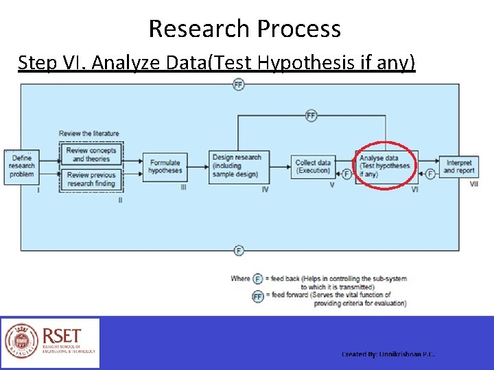
Research Process Step VI. Analyze Data(Test Hypothesis if any)

Data analysis methods • Qualitative data analysis- Analysis of content of interview to identify the main themes that emerge from responses given by respondents. This is done in 4 steps – Identify main themes. – Assign codes to the main themes. – Classify responses into the main themes. – Integrate themes and responses into the text of your report. 6

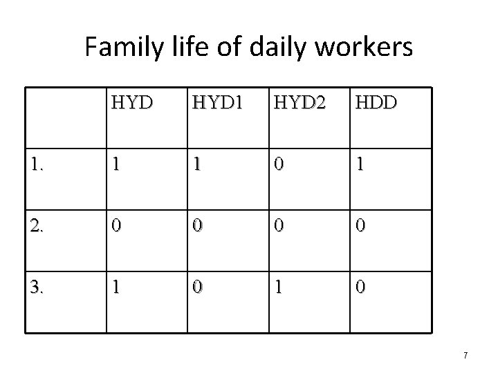
Family life of daily workers HYD 1 HYD 2 HDD 1. 1 1 0 1 2. 0 0 3. 1 0 7

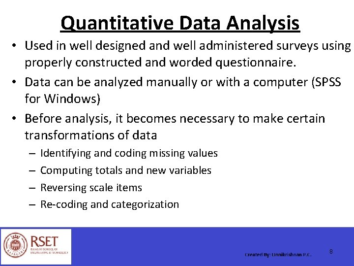
Quantitative Data Analysis • Used in well designed and well administered surveys using properly constructed and worded questionnaire. • Data can be analyzed manually or with a computer (SPSS for Windows) • Before analysis, it becomes necessary to make certain transformations of data – – Identifying and coding missing values Computing totals and new variables Reversing scale items Re-coding and categorization 8

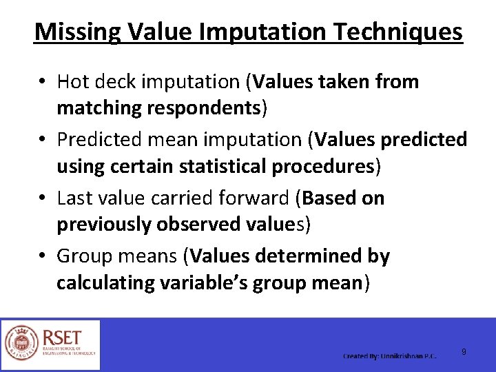
Missing Value Imputation Techniques • Hot deck imputation (Values taken from matching respondents) • Predicted mean imputation (Values predicted using certain statistical procedures) • Last value carried forward (Based on previously observed values) • Group means (Values determined by calculating variable’s group mean) 9

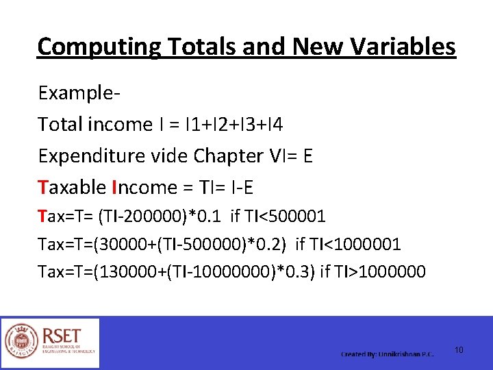
Computing Totals and New Variables Example. Total income I = I 1+I 2+I 3+I 4 Expenditure vide Chapter VI= E Taxable Income = TI= I-E Tax=T= (TI-200000)*0. 1 if TI<500001 Tax=T=(30000+(TI-500000)*0. 2) if TI<1000001 Tax=T=(130000+(TI-10000000)*0. 3) if TI>1000000 10

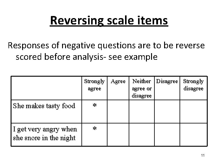
Reversing scale items Responses of negative questions are to be reverse scored before analysis- see example Strongly Agree agree She makes tasty food * I get very angry when she snore in the night * Neither Disagree Strongly agree or disagree 11

Re-Coding Variables • Turning a continuous variable into categorical variable or collapsing some observations into ranges Example – age, income etc. 12

Data Analysis Contd……. Generally, analysis of data involves one or more of the following tasks 1. Computation of descriptive statistics 2. Regression analysis 3. Correlation analysis 4. Testing hypotheses 5. Factor analysis 6. Discriminant analysis 7. Conjoint analysis 13

Data analysis • Descriptive statistics- It allow the researcher to describe the data and examine relationship between the variables. Used to summarize a study sample prior to analyzing a study’s primary hypotheses (frequency tables, histograms, measures of central tendency, dispersion, correlation, skewness) • Inferential statistics- It allow the researcher to examine causal relationships (t-test, ANOVA, chi -square and regression) 14

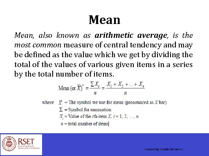
Measures of central tendency Amongst the measures of central tendency, the three most important ones are the arithmetic average or mean, median and mode. Geometric mean and harmonic mean are also sometimes used.

Mean, also known as arithmetic average, is the most common measure of central tendency and may be defined as the value which we get by dividing the total of the values of various given items in a series by the total number of items.

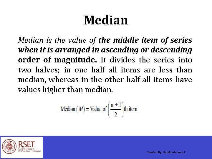
Median is the value of the middle item of series when it is arranged in ascending or descending order of magnitude. It divides the series into two halves; in one half all items are less than median, whereas in the other half all items have values higher than median.

Mode is the most commonly or frequently occurring value in a series. The mode in a distribution is that item around which there is maximum concentration. In general, mode is the size of the item which has the maximum frequency, but at items such an item may not be mode on account of the effect of the frequencies of the neighboring items. Like median, mode is a positional average and is not affected by the values of extreme items. it is, therefore, useful in all situations where we want to eliminate the effect of extreme variations.

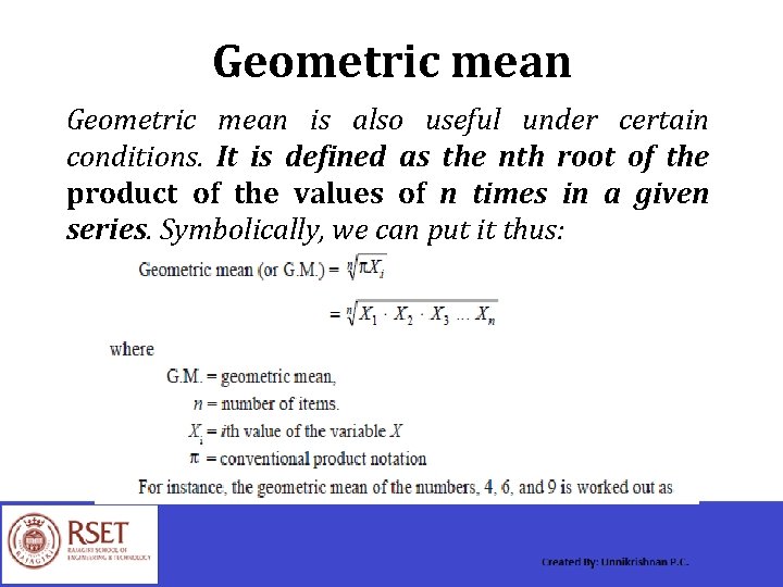
Geometric mean is also useful under certain conditions. It is defined as the nth root of the product of the values of n times in a given series. Symbolically, we can put it thus:

MEASURES OF DISPERSION An averages can represent a series only as best as a single figure can, but it certainly cannot reveal the entire story of any phenomenon under study. Specially it fails to give any idea about the scatter of the values of items of a variable in the series around the true value of average. In order to measure this scatter, statistical devices called measures of dispersion are calculated. Important measures of dispersion are (a) range, (b) mean deviation, and (c) standard deviation.

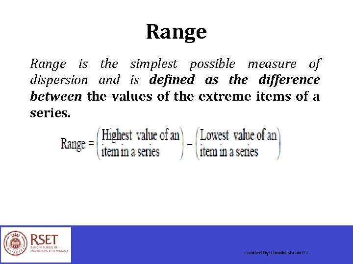
Range is the simplest possible measure of dispersion and is defined as the difference between the values of the extreme items of a series.

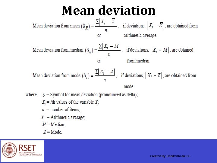
Mean deviation is the average of difference of the values of items from some average of the series. Such a difference is technically described as deviation. In calculating mean deviation we ignore the minus sign of deviations while taking their total for obtaining the mean deviation.

Mean deviation

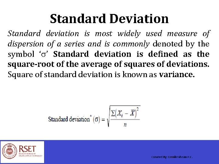
Standard Deviation Standard deviation is most widely used measure of dispersion of a series and is commonly denoted by the symbol ‘ ’ Standard deviation is defined as the square-root of the average of squares of deviations. Square of standard deviation is known as variance.

Example The owner of a restaurant is interested in how much people spend at the restaurant. He examines 10 randomly selected receipts for parties of four and writes down the following data (In Rupees) 440, 500, 380, 960, 420, 470, 400, 390, 460, 500 Calculate Mean, Median, Mode, Range, Variance and Sandard Deviation

SAMPLING DISTRIBUTIONS Some important sampling distributions, which are commonly used (1) sampling distribution of mean (2) sampling distribution of proportion (3) student’s ‘t’ distribution (4) F distribution (5) Chi-square distribution.

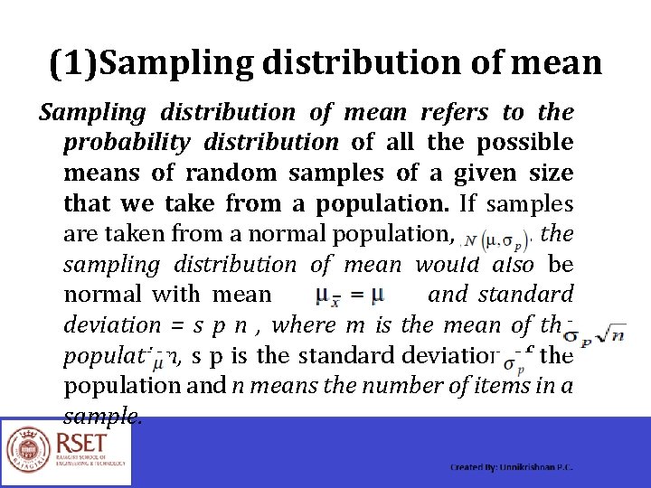
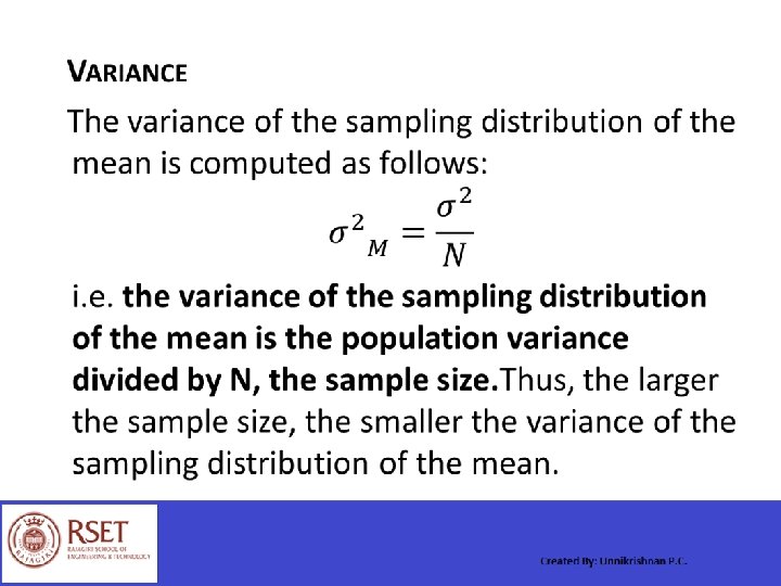
(1)Sampling distribution of mean refers to the probability distribution of all the possible means of random samples of a given size that we take from a population. If samples are taken from a normal population, , the sampling distribution of mean would also be normal with mean and standard deviation = s p n , where m is the mean of the population, s p is the standard deviation of the population and n means the number of items in a sample.

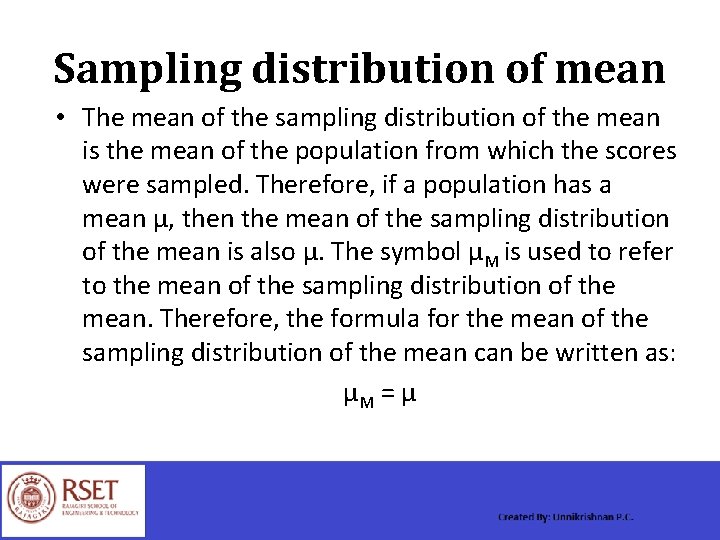
Sampling distribution of mean • The mean of the sampling distribution of the mean is the mean of the population from which the scores were sampled. Therefore, if a population has a mean μ, then the mean of the sampling distribution of the mean is also μ. The symbol μM is used to refer to the mean of the sampling distribution of the mean. Therefore, the formula for the mean of the sampling distribution of the mean can be written as: μM = μ

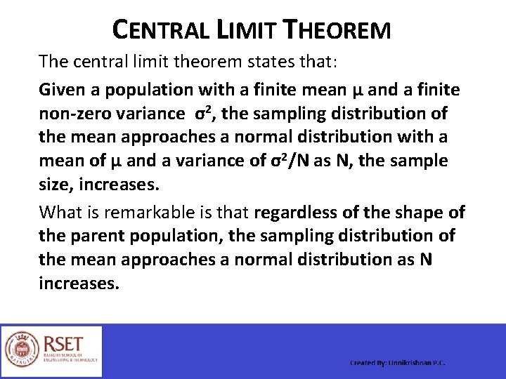
CENTRAL LIMIT THEOREM The central limit theorem states that: Given a population with a finite mean μ and a finite non-zero variance σ2, the sampling distribution of the mean approaches a normal distribution with a mean of μ and a variance of σ2/N as N, the sample size, increases. What is remarkable is that regardless of the shape of the parent population, the sampling distribution of the mean approaches a normal distribution as N increases.

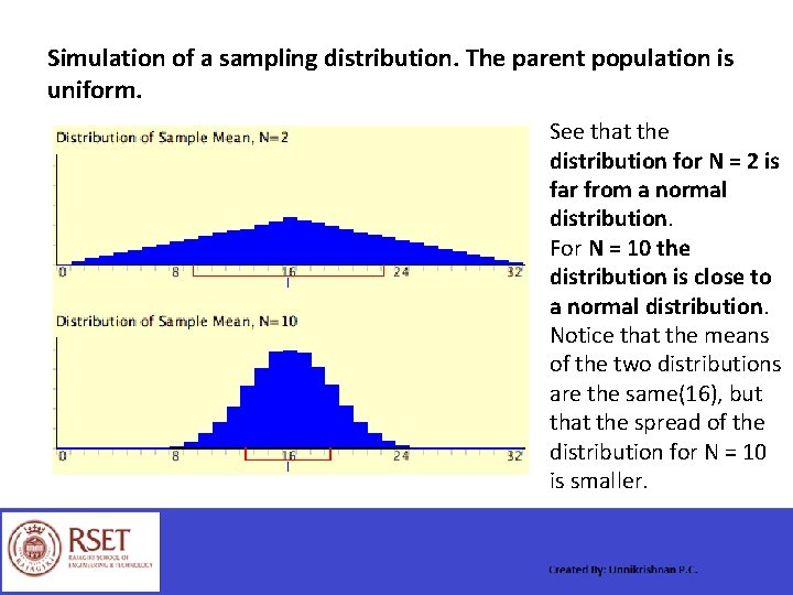
Simulation of a sampling distribution. The parent population is uniform. See that the distribution for N = 2 is far from a normal distribution. For N = 10 the distribution is close to a normal distribution. Notice that the means of the two distributions are the same(16), but that the spread of the distribution for N = 10 is smaller.

Sampling distribution of mean When sampling is from a population which is not normal (may be positively or negatively skewed), even then, as per the central limit theorem, the sampling distribution of mean tends quite closer to the normal distribution, provided the number of sample items is large.

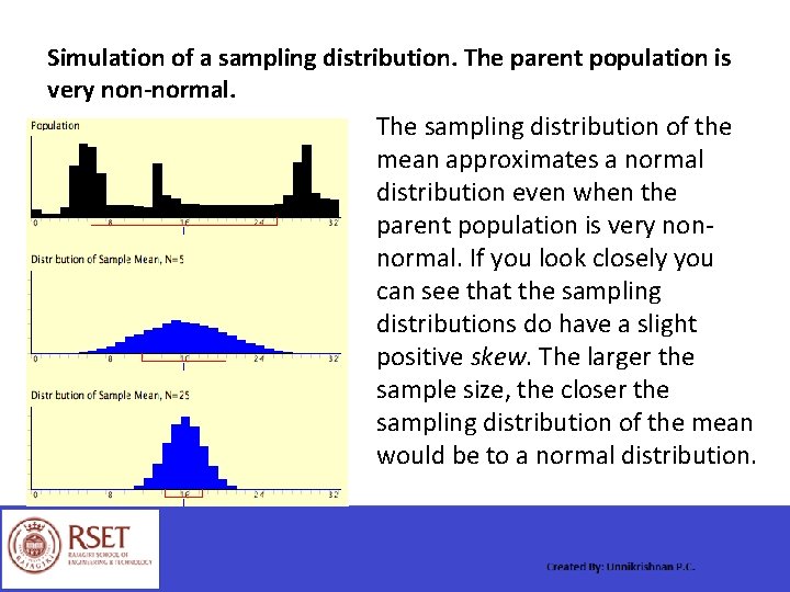
Simulation of a sampling distribution. The parent population is very non-normal. The sampling distribution of the mean approximates a normal distribution even when the parent population is very nonnormal. If you look closely you can see that the sampling distributions do have a slight positive skew. The larger the sample size, the closer the sampling distribution of the mean would be to a normal distribution.

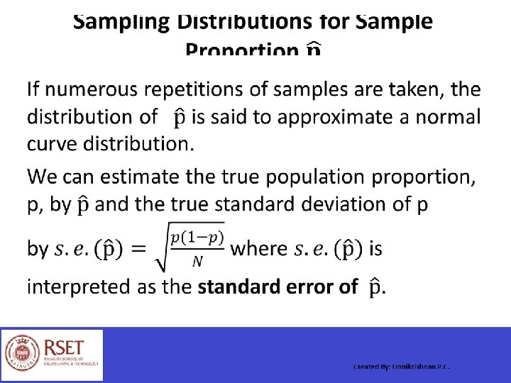
(2) Sampling Distribution of Proportion Population Proportion ( ) Population proportion is part of a population with a particular attribute, expressed as a fraction, decimal or percentage of the whole population. For a finite population, the population proportion is the number of members in the population with a particular attribute divided by the number of members in the population.

• Sample Proportions …. .

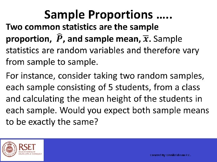
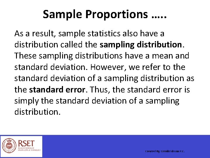
Sample Proportions …. . As a result, sample statistics also have a distribution called the sampling distribution. These sampling distributions have a mean and standard deviation. However, we refer to the standard deviation of a sampling distribution as the standard error. Thus, the standard error is simply the standard deviation of a sampling distribution.

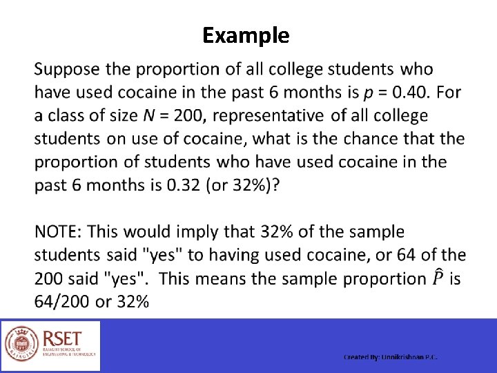
Example

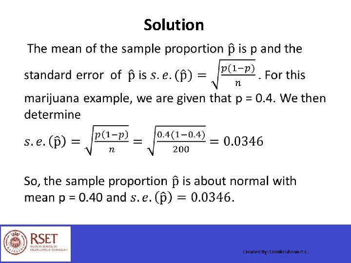
Solution

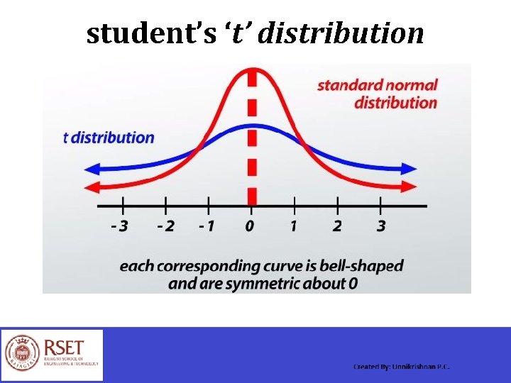
student’s ‘t’ distribution

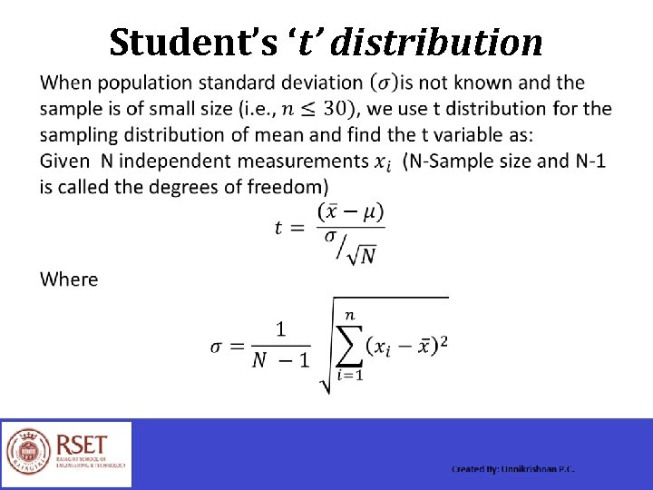
Student’s ‘t’ distribution

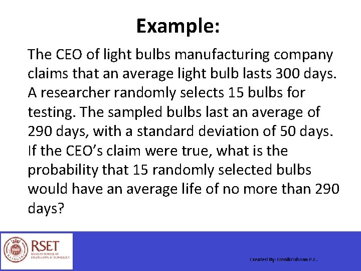
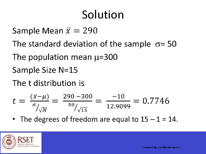
Example: The CEO of light bulbs manufacturing company claims that an average light bulb lasts 300 days. A researcher randomly selects 15 bulbs for testing. The sampled bulbs last an average of 290 days, with a standard deviation of 50 days. If the CEO’s claim were true, what is the probability that 15 randomly selected bulbs would have an average life of no more than 290 days?

Solution •

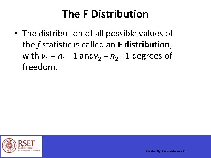
F distribution • The F distribution is the probability distribution associated with the f statistic.

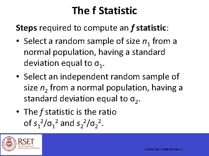
The f Statistic Steps required to compute an f statistic: • Select a random sample of size n 1 from a normal population, having a standard deviation equal to σ1. • Select an independent random sample of size n 2 from a normal population, having a standard deviation equal to σ2. • The f statistic is the ratio of s 12/σ12 and s 22/σ22.

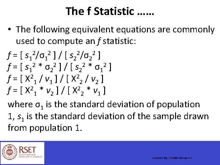
The f Statistic …… • The following equivalent equations are commonly used to compute an f statistic: f = [ s 12/σ12 ] / [ s 22/σ22 ] f = [ s 1 2 * σ 2 2 ] / [ s 2 2 * σ 1 2 ] f = [ Χ 21 / v 1 ] / [ Χ 22 / v 2 ] f = [ Χ 21 * v 2 ] / [ Χ 22 * v 1 ] where σ1 is the standard deviation of population 1, s 1 is the standard deviation of the sample drawn from population 1.

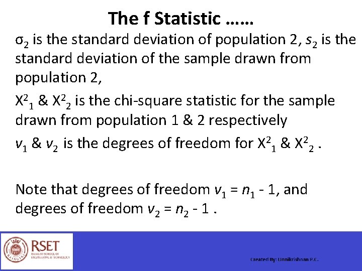
The f Statistic …… σ2 is the standard deviation of population 2, s 2 is the standard deviation of the sample drawn from population 2, Χ 21 & Χ 22 is the chi-square statistic for the sample drawn from population 1 & 2 respectively v 1 & v 2 is the degrees of freedom for Χ 21 & Χ 22. Note that degrees of freedom v 1 = n 1 - 1, and degrees of freedom v 2 = n 2 - 1.

The F Distribution • The distribution of all possible values of the f statistic is called an F distribution, with v 1 = n 1 - 1 andv 2 = n 2 - 1 degrees of freedom.

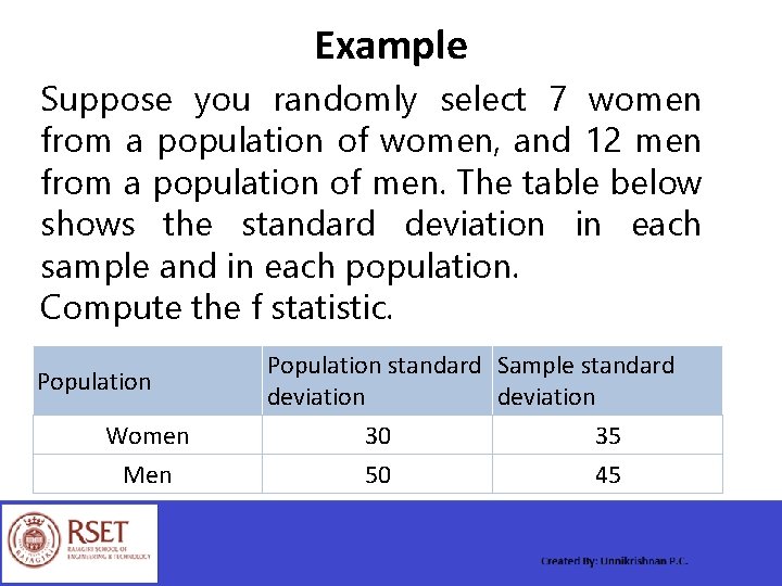
Example Suppose you randomly select 7 women from a population of women, and 12 men from a population of men. The table below shows the standard deviation in each sample and in each population. Compute the f statistic. Population Women Men Population standard Sample standard deviation 30 50 35 45

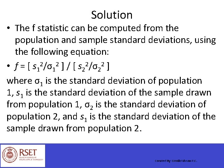
Solution • The f statistic can be computed from the population and sample standard deviations, using the following equation: • f = [ s 12/σ12 ] / [ s 22/σ22 ] where σ1 is the standard deviation of population 1, s 1 is the standard deviation of the sample drawn from population 1, σ2 is the standard deviation of population 2, and s 1 is the standard deviation of the sample drawn from population 2.

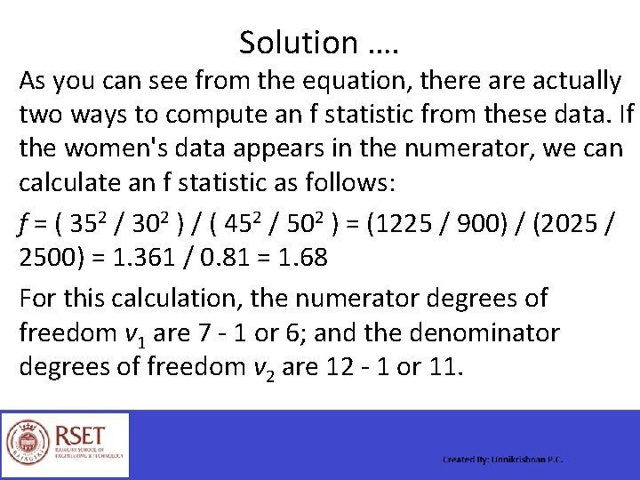
Solution …. As you can see from the equation, there actually two ways to compute an f statistic from these data. If the women's data appears in the numerator, we can calculate an f statistic as follows: f = ( 352 / 302 ) / ( 452 / 502 ) = (1225 / 900) / (2025 / 2500) = 1. 361 / 0. 81 = 1. 68 For this calculation, the numerator degrees of freedom v 1 are 7 - 1 or 6; and the denominator degrees of freedom v 2 are 12 - 1 or 11.

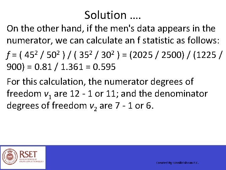
Solution …. On the other hand, if the men's data appears in the numerator, we can calculate an f statistic as follows: f = ( 452 / 502 ) / ( 352 / 302 ) = (2025 / 2500) / (1225 / 900) = 0. 81 / 1. 361 = 0. 595 For this calculation, the numerator degrees of freedom v 1 are 12 - 1 or 11; and the denominator degrees of freedom v 2 are 7 - 1 or 6.

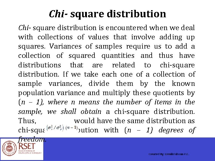
Chi- square distribution is encountered when we deal with collections of values that involve adding up squares. Variances of samples require us to add a collection of squared quantities and thus have distributions that are related to chi-square distribution. If we take each one of a collection of sample variances, divide them by the known population variance and multiply these quotients by (n – 1), where n means the number of items in the sample, we shall obtain a chi-square distribution. Thus, would have the same distribution as chi-square distribution with (n – 1) degrees of freedom.