Research Methodology Dr Unnikrishnan P C Professor EEE

Research Methodology Dr. Unnikrishnan P. C. Professor, EEE

Dr. Unnikrishnan P. C. l l l BTech. : EEE, NSS College of Engineering, 1981 -85. MTech: Control & Instrumentation, IIT Bombay, 1990 -92. Ph. D. : EEE, Karpagam University, Coimbatore, 2010 -2016.

Dr. Unnikrishnan P. C. l l l 1986 -1996 : Assistant Professor and Associate Professor, Rajasthan Technical University, Kota, India 1996 -2016 : Assistant Professor, Academic Coordinator, Registrar, Head of Section and Head of the Department at Colleges of Technology, Ministry of Manpower, Muscat, Sultanate of Oman. 2016 : Professor, EEE, RSET

Module III q Descriptive and Inferential Statistics

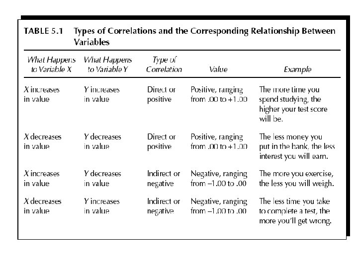
Correlation • The degree of relationship between the variables under consideration is measure through the correlation analysis. • The measure of correlation called the correlation coefficient • The degree of relationship is expressed by coefficient which range from correlation ( -1 ≤ r ≥ +1) • The direction of change is indicated by a sign. • The correlation analysis enable us to have an idea about the degree & direction of the relationship between the two variables under study.

Conceptualizing Correlation Measuring Development Weak GPD POP WEIGHT Strong GDP EDUCATION Correlation will be associated with what type of validity?

Rules of Thumb Size of correlation coefficient. 8 - 1. 0 General Interpretation . 6 -. 8 Strong . 4 -. 6 Moderate . 2 -. 4 Weak . 0 -. 2 Very Weak or no relationship Very Strong The strength of the correlation depends on how many data points in the scatter plot are near or far in a pattern. This is similar to error in the data, which comes from other explanations

Methods of Studying Correlation • Scatter Diagram Method • Graphic Method • Karl Pearson’s Coefficient of Correlation • Method of Least Squares

Scatter Diagram Method • Scatter Diagram is a graph of observed plotted points where each points represents the values of X & Y as a coordinate. It portrays the relationship between these two variables graphically.

The shape of the relationship can be depicted in scatterplots. What type of relationship do you see?

A perfect positive correlation

High Degree of positive correlation • Positive relationship

Degree of correlation • Moderate Positive Correlation r = + 0. 4 Shoe Size Weight

Degree of correlation • Perfect Negative Correlation

Degree of correlation • Moderate Negative Correlation

Degree of correlation • No Correlation (horizontal line) r = 0. 0 IQ Height

Scatter Plots and Types of Correlation Strong, negative relationship but non-linear!

Karl Pearson's Coefficient of Correlation • Pearson’s ‘r’ is the most common correlation coefficient. • Karl Pearson’s Coefficient of Correlation denoted by- ‘r’ The coefficient of correlation ‘r’ measure the degree of linear relationship between two variables say x & y.

Correlation Coefficient “r” A measure of the strength and direction of a linear relationship between two variables The range of r is from – 1 to 1. If r is close to – 1 there is a strong negative correlation. If r is close to 0 there is no linear correlation. If r is close to 1 there is a strong positive correlation.

Outliers. . . Outliers are dangerous Here we have a spurious correlation of r=0. 68 without IBM, r=0. 48 without IBM & GE, r=0. 21

Application Find the Correlation between Absence and Final Grade Final Absences Grade 95 90 85 80 75 70 65 60 55 50 45 40 0 2 4 6 8 10 Absences X 12 14 16 x 8 2 5 12 15 9 6 y 78 92 90 58 43 74 81

Computation of r 1 2 3 4 5 6 7 x y 8 2 5 12 15 9 6 78 92 90 58 43 74 81 57 516 xy 624 184 450 696 645 666 486 x 2 64 4 25 144 225 81 36 y 2 6084 8464 8100 3364 1849 5476 6561 3751 579 39898

Hypothesis 24

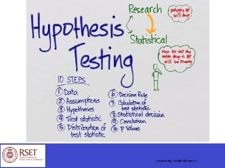
Hypothesis Testing 26

Hypothesis Testing 27

Hypothesis Testing 28

Hypothesis Testing 34

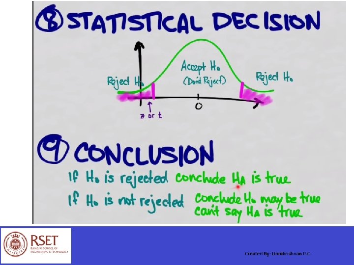
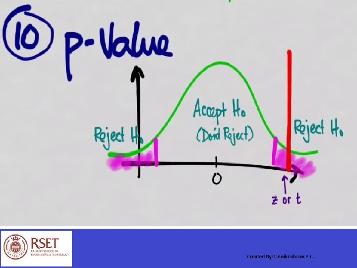
Hypothesis Testing Steps 11. Check whether to reject the null hypothesis by comparing p-value to (Level of Significance) 12. Conclusion in words

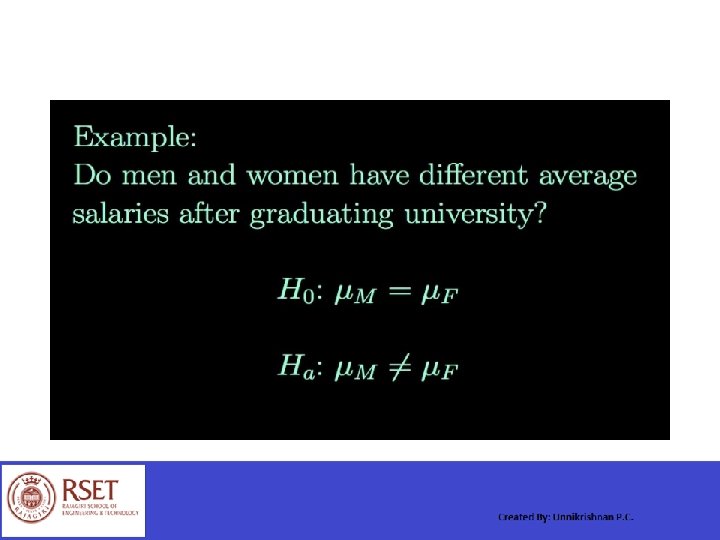
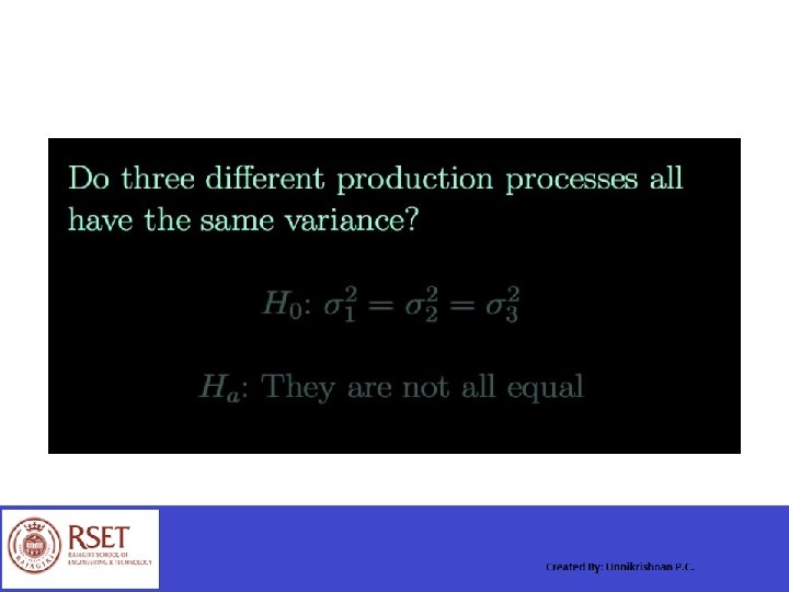
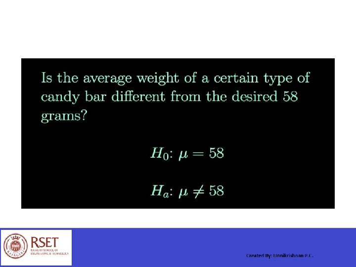
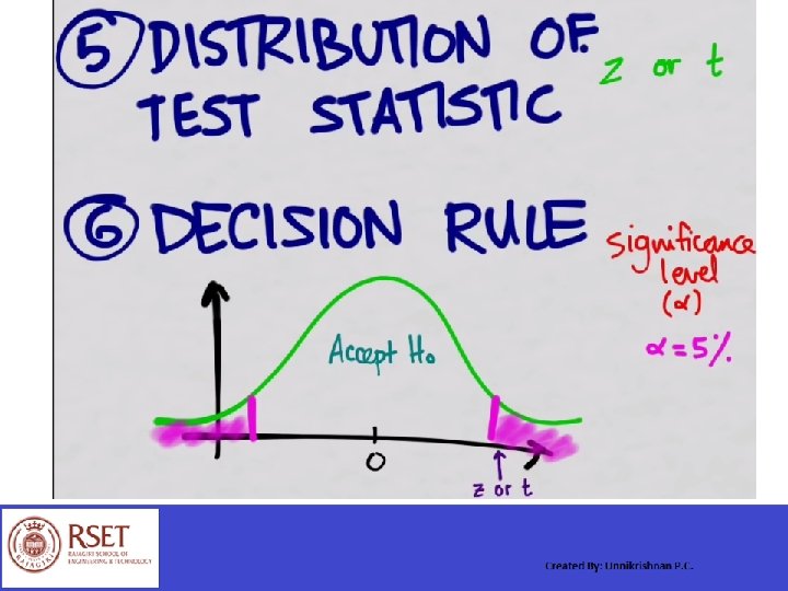
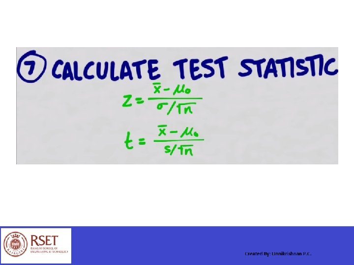
Hypothesis Testing Steps 1. The null and alternative hypotheses 2. Level of significance α 3. Test statistics 4. Compute the p-value 5. Check whether to reject the null hypothesis by comparing p-value to α 6. Conclusion in words

Hypothesis Test for Significance r is the correlation coefficient for the sample. The correlation coefficient for the population is (rho). For a two tail test for significance: (The correlation is not significant) (The correlation is significant) The sampling distribution for r is a t-distribution with n – 2 d. f. Standardized test statistic

Example 1. Data: The correlation between the number of times absent and a final grade r = – 0. 975. There were seven pairs of data. Test the significance of this correlation = 0. 01. 2. Assumptions: Normal Distribution 3. Hypothesis. (The correlation is not significant) (The correlation is significant) 4. Test Statistics. A t-distribution with 5 degrees of freedom

Example ……. . 5. Distribution of Test Statistics. Normal Distribution 6. Decision Rule: State the level of significance. = 0. 01 7. Calculation of Test Statistics 9. Conclusion 10. P-Values

7. Calculation of Test Statistics Rejection Regions Critical Values ± t 0 t – 4. 032 0 4. 032 Find the critical value. Find the rejection region. Find the test statistic. dfp 0. 40 0. 25 0. 10 0. 05 0. 025 0. 01 0. 005 0. 0005 1 0. 324920 1. 000000 3. 077684 6. 313752 12. 70620 31. 82052 63. 65674 636. 6192 2 0. 288675 0. 816497 1. 885618 2. 919986 4. 30265 6. 96456 9. 92484 31. 5991 3 0. 276671 0. 764892 1. 637744 2. 353363 3. 18245 4. 54070 5. 84091 12. 9240 4 0. 270722 0. 740697 1. 533206 2. 131847 2. 77645 3. 74695 4. 60409 8. 6103 5 0. 267181 0. 726687 1. 475884 2. 015048 2. 57058 3. 36493 4. 03214 6. 8688

t – 4. 032 0 +4. 032 8. Statistical decision. t = – 9. 811 falls in the rejection region. Reject the null hypothesis. 9. Conclusion. There is a significant negative correlation between the number of times absent and final grades. 10. P-Values

The Line of Regression § Regression indicates the degree to which the variation in one variable X, is related to or can be explained by the variation in another variable Y § Once you know there is a significant linear correlation, you can write an equation describing the relationship between the x and y variables. § This equation is called the line of regression or least squares line. The equation of a line may be written as y = mx + b where m is the slope of the line and b is the yintercept. The line of regression is: The slope m is: The y-intercept is:

(xi, yi) = a data point = a point on the line with the same x-value = a residual Best fitting straight line 260 revenue 250 240 230 220 210 200 190 180 1. 5 2. 0 Ad $ 2. 5 3. 0

1 2 3 4 5 6 7 x 8 2 5 12 15 9 6 xy y 78 92 90 58 43 74 81 624 184 450 696 645 666 486 57 516 3751 x 2 64 4 25 144 225 81 36 y 2 6084 8464 8100 3364 1849 5476 6561 579 39898 The line of regression is: Write the equation of the line of regression with x = number of absences and y = final grade. Calculate m and b. = – 3. 924 x + 105. 667

The Line of Regression Final Grade m = – 3. 924 and b = 105. 667 The line of regression is: 95 90 85 80 75 70 65 60 55 50 45 40 0 2 4 6 8 10 12 14 16 Absences Note that the point = (8. 143, 73. 714) is on the line.

Predicting y Values The regression line can be used to predict values of y for values of x falling within the range of the data. The regression equation for number of times absent and final grade is: = – 3. 924 x + 105. 667 Use this equation to predict the expected grade for a student with (a) 3 absences (b) 12 absences (a) = – 3. 924(3) + 105. 667 = 93. 895 (b) = – 3. 924(12) + 105. 667 = 58. 579

Strength of the Association The coefficient of determination, r 2, measures the strength of the association and is the ratio of explained variation in y to the total variation in y. The correlation coefficient of number of times absent and final grade is r = – 0. 975. The coefficient of determination is r 2 = (– 0. 975)2 = 0. 9506. Interpretation: About 95% of the variation in final grades can be explained by the number of times a student is absent. The other 5% is unexplained and can be due to sampling error or other variables such as intelligence, amount of time studied, etc.

Correlation Analysis • We focus here on the Pearson productmoment correlation, which is used for continuous measures (ratio, interval = scalar) • Spearman’s rho Kendall’s Tau-b used to compare ordered variables

Correlation and Causation • We want to know how two variables are related to, overlap with, each other • If one variable causes another, it will be correlated with it. • However, some correlations are spurious and association does not automatically mean causation.

Correlating Developmental factors

Significance of Variables • We can also estimate whether certain variables are important. We do this by ascertaining statistical significance. • Our key question is: What is the probability that an estimate is produced by random chance and there is no relationship between X and Y variables?

Significance of Variables • We measure statistical significance by the probability that we are observing is wrong (generated by random chance). • A significance level of. 05 is conventional. This means that if the significance level is. 05, there is a 5 percent chance that our results were generated randomly. A. 01 level means there is a 1 percent chance.

Another Example

Limitation of correlation coefficients • • • They tell us how strongly two variables are related May capture causation between variables but cannot differentiate from spurious ones. However, r coefficients are limited because they cannot tell anything about: Marginal impact of X on Y Direction of causation when present Forecasting Because of the above Ordinary Least Square regression analysis (OLS) is most useful

Hypothesis Testing Type I and Type II Errors

Acceptance Region-Two Tailed Test Sampling Distribution of Test Statistic

Acceptance Region-One Tailed Test

Acceptance Region-One Tailed Test

Flow Diagram For Hypothesis Testing

PROCEDURE FOR HYPOTHESIS TESTING Ø Making a formal statement Ø Selecting a significance level Ø Deciding the distribution to use Ø Selecting a random sample and computing an appropriate value Ø Calculation of the probability Ø Comparing the probability

HYPOTHESIS TESTING OF MEANS

HYPOTHESIS TESTING OF MEANS

HYPOTHESIS TESTING OF MEANS

HYPOTHESIS TESTING OF MEANS