Recap Term frequency tfidf weighting The vector space

Recap Term frequency tf-idf weighting The vector space Introduction to Information Retrieval http: //informationretrieval. org IIR 6: Scoring, Term Weighting, The Vector Space Model Hinrich Schu¨tze Institute for Natural Language Processing, Universit¨at Stuttgart 2008. 05. 20 Schu¨tze: Scoring, term weighting, the vector space model 1 / 53

Recap The term vocabulary Skip pointers Phrase queries Definitions Word – A delimited string of characters as it appears in the text. Term – A “normalized” word (case, morphology, spelling etc); an equivalence class of words. Token – An instance of a word or term occurring in a document. Type – The same as a term in most cases: an equivalence class of tokens. Schu¨tze: The term vocabulary and postings lists 13 / 60

Recap The term vocabulary Skip pointers Phrase queries Recall: Inverted index construction Input: Friends, Romans, countrymen. So let it be with Caesar . . . Output: friend roman countryman so. . . Each token is a candidate for a postings entry. What are valid tokens to emit? Schu¨tze: The term vocabulary and postings lists 15 / 60

Recap The term vocabulary Skip pointers Phrase queries Stop words stop words = extremely common words which would appear to be of little value in helping select documents matching a user need Examples: a, and, are, as, at, be, by, for, from, has, he, in, is, its, of, on, that, the, to, was, were, will, with Stop word elimination used to be standard in older IR systems. But you need stop words for phrase queries, e. g. “King of Denmark” Most web search engines index stop words. Schu¨tze: The term vocabulary and postings lists 29 / 60

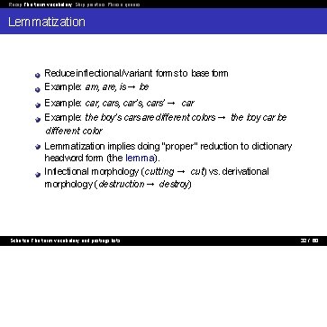
Recap The term vocabulary Skip pointers Phrase queries Lemmatization Reduce inflectional/variant forms to base form Example: am, are, is → be Example: car, cars, car’s, cars’ → car Example: the boy’s cars are different colors → the boy car be different color Lemmatization implies doing “proper” reduction to dictionary headword form (the lemma). Inflectional morphology (cutting → cut) vs. derivational morphology (destruction → destroy) Schu¨tze: The term vocabulary and postings lists 32 / 60

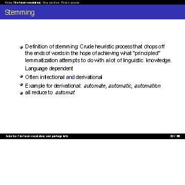
Recap The term vocabulary Skip pointers Phrase queries Stemming Definition of stemming: Crude heuristic process that chops off the ends of words in the hope of achieving what “principled” lemmatization attempts to do with a lot of linguistic knowledge. Language dependent Often inflectional and derivational Example for derivational: automate, automatic, automation all reduce to automat Schu¨tze: The term vocabulary and postings lists 33 / 60

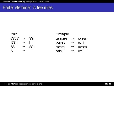
Recap The term vocabulary Skip pointers Phrase queries Porter stemmer: A few rules Rule SSES IES SS S → → SS I SS Schu¨tze: The term vocabulary and postings lists Example caresses ponies caress cats → → caress poni caress cat 35 / 60

Recap Term frequency tf-idf weighting The vector space Outline 1 Recap 2 Term frequency 3 tf-idf weighting 4 The vector space Schu¨tze: Scoring, term weighting, the vector space model 9 / 53

Recap Term frequency tf-idf weighting The vector space Scoring as the basis of ranked retrieval We wish to return in order the documents most likely to be useful to the searcher. How can we rank-order the documents in the collection with respect to a query? Assign a score – say in [0, 1] – to each document This score measures how well document and query “match”. Schu¨tze: Scoring, term weighting, the vector space model 12 / 53

Recap Term frequency tf-idf weighting The vector space Query-document matching scores We need a way of assigning a score to a query/document pair. Let’s start with a one-term query. If the query term does not occur in the document: score should be 0. The more frequent the query term in the document, the higher the score Schu¨tze: Scoring, term weighting, the vector space model 13 / 53

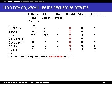
Recap Term frequency tf-idf weighting The vector space From now on, we will use the frequencies of terms Anthony and Cleopatr a 157 4 232 0 57 2 2 Julius Caesar The Tempest Hamlet Anthony 73 0 0 Brutus 157 0 2 Caesar 227 0 2 Calpurnia 10 0 0 Cleopatra 0 0 0 mercy 0 3 8 worser 0 1 1. . . Each document is represented by a count vector ∈ N|V |. Schu¨tze: Scoring, term weighting, the vector space model Othello Macbeth 0 0 1 0 0 5 1 1 0 0 8 5 . . . 18 / 53

Recap Term frequency tf-idf weighting The vector space Bag of words model We do not consider the order of words in a document. John is quicker than Mary and Mary is quicker than John are represented the same way. This is called a bag of words model. Schu¨tze: Scoring, term weighting, the vector space model 19 / 53

Recap Term frequency tf-idf weighting The vector space Term frequency tf The term frequency tft , d of term t in document d is defined as the number of times that t occurs in d. We want to use tf when computing query-document match scores. But how? Schu¨tze: Scoring, term weighting, the vector space model 20 / 53

Recap Term frequency tf-idf weighting The vector space Term frequency tf The term frequency tft , d of term t in document d is defined as the number of times that t occurs in d. We want to use tf when computing query-document match scores. But how? Raw term frequency is not what we want. A document with 10 occurrences of the term is more relevant than a document with one occurrence of the term. But not 10 times more relevant. Relevance does not increase proportionally with term frequency. Schu¨tze: Scoring, term weighting, the vector space model 20 / 53

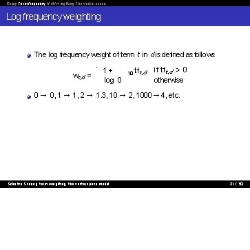
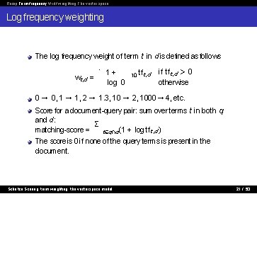
Recap Term frequency tf-idf weighting The vector space Log frequency weighting The log frequency weight of term t in d is defined as follows. wt, d = 1+ log 0 10 tf t, d if tft , d > 0 otherwise 0 → 0, 1 → 1, 2 → 1. 3, 10 → 2, 1000 → 4, etc. Schu¨tze: Scoring, term weighting, the vector space model 21 / 53

Recap Term frequency tf-idf weighting The vector space Log frequency weighting The log frequency weight of term t in d is defined as follows. wt, d = 1+ log 0 10 tf t, d if tft , d > 0 otherwise 0 → 0, 1 → 1, 2 → 1. 3, 10 → 2, 1000 → 4, etc. Score for a document-query pair: sum over terms t in both q and d : Σ matching-score = t∈q∩d(1 + log tft , d ) Schu¨tze: Scoring, term weighting, the vector space model 21 / 53

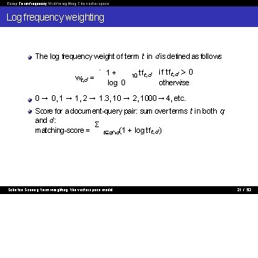
Recap Term frequency tf-idf weighting The vector space Log frequency weighting The log frequency weight of term t in d is defined as follows. wt, d = 1+ log 0 10 tf t, d if tft , d > 0 otherwise 0 → 0, 1 → 1, 2 → 1. 3, 10 → 2, 1000 → 4, etc. Score for a document-query pair: sum over terms t in both q and d : Σ matching-score = t∈q∩d(1 + log tft , d ) The score is 0 if none of the query terms is present in the document. Schu¨tze: Scoring, term weighting, the vector space model 21 / 53

Recap Term frequency tf-idf weighting The vector space Outline 1 Recap 2 Term frequency 3 tf-idf weighting 4 The vector space Schu¨tze: Scoring, term weighting, the vector space model 22 / 53

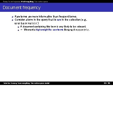
Recap Term frequency tf-idf weighting The vector space Document frequency Rare terms are more informative than frequent terms. Consider a term in the query that is rare in the collection (e. g. , arachnocentric) A document containing this term is very likely to be relevant. → We want a high weight for rare terms like a r a c h n o c e n t r i c. Schu¨tze: Scoring, term weighting, the vector space model 23 / 53

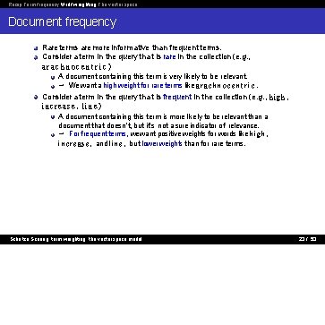
Recap Term frequency tf-idf weighting The vector space Document frequency Rare terms are more informative than frequent terms. Consider a term in the query that is rare in the collection (e. g. , arachnocentric) A document containing this term is very likely to be relevant. → We want a high weight for rare terms like a r a c h n o c e n t r i c. Consider a term in the query that is frequent in the collection (e. g. , h i g h , increase, line) A document containing this term is more likely to be relevant than a document that doesn’t, but it’s not a sure indicator of relevance. → For frequent terms, we want positive weights for words like high , i n c r e a s e , and l i n e , but lower weights than for rare terms. Schu¨tze: Scoring, term weighting, the vector space model 23 / 53

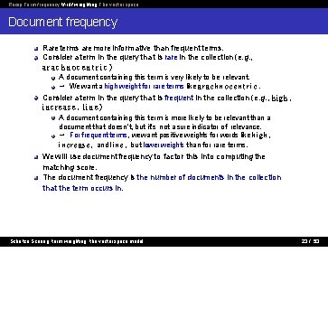
Recap Term frequency tf-idf weighting The vector space Document frequency Rare terms are more informative than frequent terms. Consider a term in the query that is rare in the collection (e. g. , arachnocentric) A document containing this term is very likely to be relevant. → We want a high weight for rare terms like a r a c h n o c e n t r i c. Consider a term in the query that is frequent in the collection (e. g. , h i g h , increase, line) A document containing this term is more likely to be relevant than a document that doesn’t, but it’s not a sure indicator of relevance. → For frequent terms, we want positive weights for words like high , i n c r e a s e , and l i n e , but lower weights than for rare terms. We will use document frequency to factor this into computing the matching score. The document frequency is the number of documents in the collection that the term occurs in. Schu¨tze: Scoring, term weighting, the vector space model 23 / 53

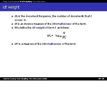
Recap Term frequency tf-idf weighting The vector space idf weight dft is the document frequency, the number of documents that t occurs in. df is an inverse measure of the informativeness of the term. We define the idf weight of term t as follows: idft = log 10 N df t idf is a measure of the informativeness of the term. Schu¨tze: Scoring, term weighting, the vector space model 24 / 53

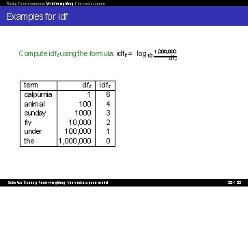
Recap Term frequency tf-idf weighting The vector space Examples for idf Compute idft using the formula: idft = log 10 1, 000 df t dft term calpurnia 1 animal 100 sunday 1000 fly 10, 000 under 100, 000 the 1, 000 idft 6 4 3 2 1 0 Schu¨tze: Scoring, term weighting, the vector space model 25 / 53

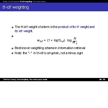
Recap Term frequency tf-idf weighting The vector space tf-idf weighting The tf-idf weight of a term is the product of its tf weight and its idf weight. wt, d = (1 + log tft , d ) ·log N df t Best known weighting scheme in information retrieval Note: the “ - ” in tf-idf is a hyphen, not a minus sign! Schu¨tze: Scoring, term weighting, the vector space model 28 / 53

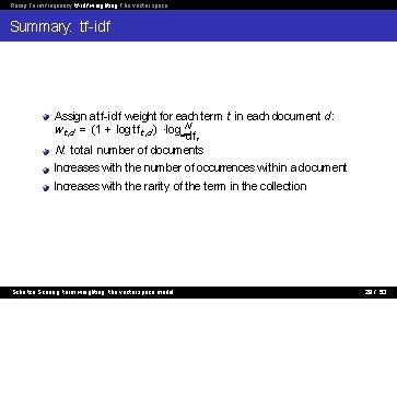
Recap Term frequency tf-idf weighting The vector space Summary: tf-idf Assign a tf-idf weight for each term t in each document d : wt, d = (1 + log tft , d ) ·log N dft N: total number of documents Increases with the number of occurrences within a document Increases with the rarity of the term in the collection Schu¨tze: Scoring, term weighting, the vector space model 29 / 53

Recap Term frequency tf-idf weighting The vector space Outline 1 Recap 2 Term frequency 3 tf-idf weighting 4 The vector space Schu¨tze: Scoring, term weighting, the vector space model 31 / 53

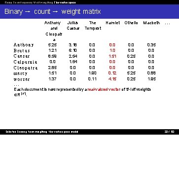
Recap Term frequency tf-idf weighting The vector space Binary → count → weight matrix Anthony and Cleopatr a 5. 25 1. 21 8. 59 0. 0 2. 85 1. 51 1. 37 Julius Caesar The Tempest Hamlet Othello Macbeth . . . Anthony 3. 18 0. 0 0. 35 Brutus 6. 10 0. 0 1. 0 0. 0 Caesar 2. 54 0. 0 1. 51 0. 25 0. 0 Calpurnia 1. 54 0. 0 Cleopatra 0. 0 0. 0 mercy 0. 0 1. 90 0. 12 5. 25 0. 88 worser 0. 0 0. 11 4. 15 0. 25 1. 95. . . Each document is now represented by a real-valued vector of tf-idf weights ∈R|V |. Schu¨tze: Scoring, term weighting, the vector space model 32 / 53

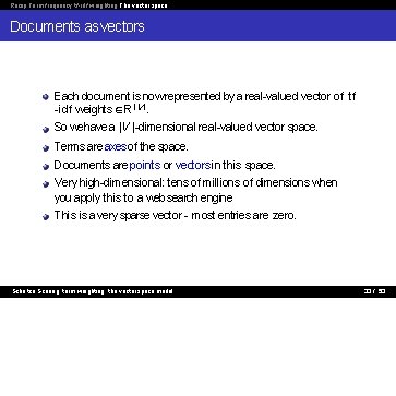
Recap Term frequency tf-idf weighting The vector space Documents as vectors Each document is now represented by a real-valued vector of tf -idf weights ∈ R|V |. So we have a |V |-dimensional real-valued vector space. Terms are axes of the space. Documents are points or vectors in this space. Very high-dimensional: tens of millions of dimensions when you apply this to a web search engine This is a very sparse vector - most entries are zero. Schu¨tze: Scoring, term weighting, the vector space model 33 / 53

Recap Term frequency tf-idf weighting The vector space Queries as vectors Key idea 1: do the same for queries: represent them as vectors in the space Key idea 2: Rank documents according to their proximity to the query Schu¨tze: Scoring, term weighting, the vector space model 34 / 53

Recap Term frequency tf-idf weighting The vector space How do we formalize vector space similarity? First cut: distance between two points ( = distance between the end points of the two vectors) Euclidean distance? Schu¨tze: Scoring, term weighting, the vector space model 35 / 53

Recap Term frequency tf-idf weighting The vector space How do we formalize vector space similarity? First cut: distance between two points ( = distance between the end points of the two vectors) Euclidean distance? Euclidean distance is a bad idea. . . because Euclidean distance is large for vectors of different lengths. Schu¨tze: Scoring, term weighting, the vector space model 35 / 53

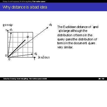
Recap Term frequency tf-idf weighting The vector space Why distance is a bad idea d 2 g o ssip 1 d 1 q The Euclidean distance of ˙qand ˙d 2 is large although the distribution of terms in the query q and the distribution of terms in the document d 2 are very similar. d 3 0 0 1 jealous Schu¨tze: Scoring, term weighting, the vector space model 36 / 53

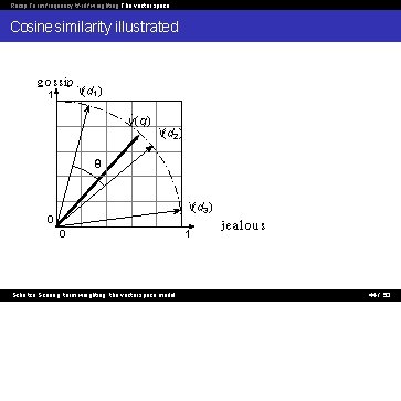
Recap Term frequency tf-idf weighting The vector space Use angle instead of distance Rank documents according to angle with query Thought experiment: take a document d and append it to itself. Call this document d ′. “Semantically” d and d ′ have the same content. The angle between the two documents is 0, corresponding to maximal similarity. The Euclidean distance between the two documents can be quite large. Schu¨tze: Scoring, term weighting, the vector space model 37 / 53

Recap Term frequency tf-idf weighting The vector space From angles to cosines The following two notions are equivalent. Rank documents according to the angle between query and document in decreasing order Rank documents according to cosine(query, document) in increasing order Cosine is a monotonically decreasing function of the angle for the interval [0◦, 180◦] Schu¨tze: Scoring, term weighting, the vector space model 38 / 53

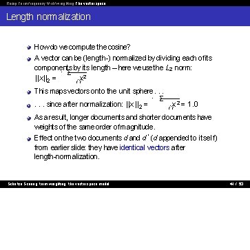
Recap Term frequency tf-idf weighting The vector space Length normalization How do we compute the cosine? A vector can be (length-) normalized by dividing each of its components. Σ by its length – here we use the L 2 norm: 2 ||x||2 = i ix This maps vectors onto the unit sphere. . Σ 2. . . since after normalization: ||x || 2 = i ix = 1. 0 As a result, longer documents and shorter documents have weights of the same order of magnitude. Effect on the two documents d and d ′ (d appended to itself) from earlier slide: they have identical vectors after length-normalization. Schu¨tze: Scoring, term weighting, the vector space model 41 / 53

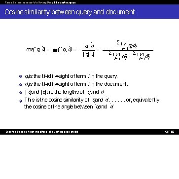
Recap Term frequency tf-idf weighting The vector space Cosine similarity between query and document cos(˙q, ˙d) = sim(˙q, ˙d) = Σ |V| qd ˙q·˙d i = 1. i i =. Σ ˙ |V | 2 Σ |V | 2 |˙q|| d| i = 1 qi i = 1 di qi is the tf-idf weight of term i in the query. di is the tf-idf weight of term i in the document. |˙q|and |˙d| are the lengths of ˙q and ˙d. This is the cosine similarity of ˙q and ˙d. . . or, equivalently, the cosine of the angle between ˙q and ˙d. Schu¨tze: Scoring, term weighting, the vector space model 42 / 53

Recap Term frequency tf-idf weighting The vector space Cosine similarity illustrated g o ssip 1 ˙v(d 1) ˙ v (q) ˙v(d 2) θ ˙v(d 3) 0 0 Schu¨tze: Scoring, term weighting, the vector space model 1 jealous 44 / 53

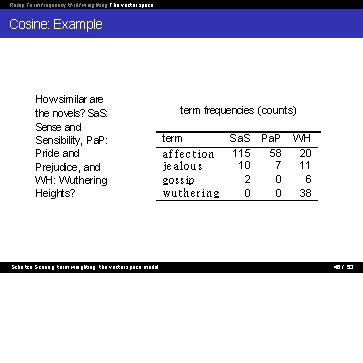
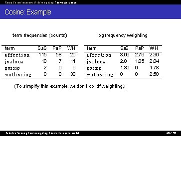
Recap Term frequency tf-idf weighting The vector space Cosine: Example How similar are the novels? Sa. S: Sense and Sensibility, Pa. P: Pride and Prejudice, and WH: Wuthering Heights? Schu¨tze: Scoring, term weighting, the vector space model term frequencies (counts) term affection jealous gossip wuthering Sa. S Pa. P 115 58 10 7 2 0 0 0 WH 20 11 6 38 45 / 53

Recap Term frequency tf-idf weighting The vector space Cosine: Example term frequencies (counts) term affection jealous gossip wuthering Sa. S 115 10 2 0 Pa. P 58 7 0 0 log frequency weighting WH 20 11 6 38 term affection jealous gossip wuthering Sa. S 3. 06 2. 0 1. 30 0 Pa. P 2. 76 1. 85 0 0 WH 2. 30 2. 04 1. 78 2. 58 (To simplify this example, we don’t do idf weighting. ) Schu¨tze: Scoring, term weighting, the vector space model 46 / 53

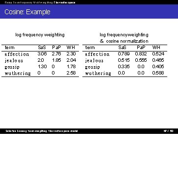
Recap Term frequency tf-idf weighting The vector space Cosine: Example log frequency weighting term affection jealous gossip wuthering Sa. S 3. 06 2. 0 1. 30 0 Pa. P 2. 76 1. 85 0 0 WH 2. 30 2. 04 1. 78 2. 58 Schu¨tze: Scoring, term weighting, the vector space model log frequency weighting & cosine normalization term Sa. S Pa. P affection 0. 789 0. 832 jealous 0. 515 0. 555 gossip 0. 335 0. 0 w u t h e r i n g 0. 0 WH 0. 524 0. 465 0. 405 0. 588 47 / 53

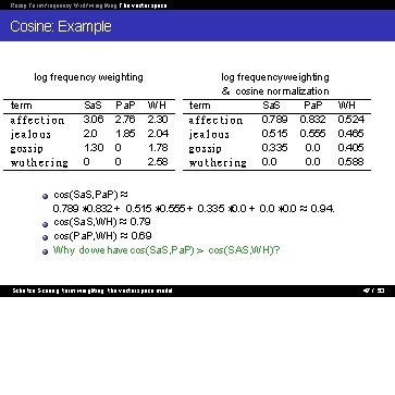
Recap Term frequency tf-idf weighting The vector space Cosine: Example log frequency weighting term affection jealous gossip wuthering Sa. S 3. 06 2. 0 1. 30 0 Pa. P 2. 76 1. 85 0 0 WH 2. 30 2. 04 1. 78 2. 58 log frequency weighting & cosine normalization term Sa. S Pa. P affection 0. 789 0. 832 jealous 0. 515 0. 555 gossip 0. 335 0. 0 w u t h e r i n g 0. 0 WH 0. 524 0. 465 0. 405 0. 588 cos(Sa. S, Pa. P) ≈ 0. 789 ∗ 0. 832 + 0. 515 ∗ 0. 555 + 0. 335 ∗ 0. 0 + 0. 0 ∗ 0. 0 ≈ 0. 94. cos(Sa. S, WH) ≈ 0. 79 cos(Pa. P, WH) ≈ 0. 69 Why do we have cos(Sa. S, Pa. P) > cos(SAS, WH)? Schu¨tze: Scoring, term weighting, the vector space model 47 / 53

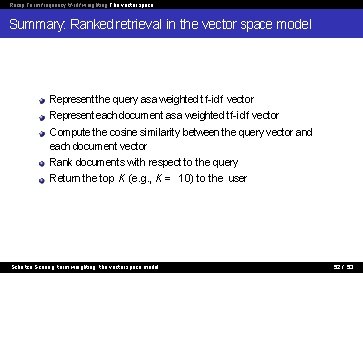
Recap Term frequency tf-idf weighting The vector space Summary: Ranked retrieval in the vector space model Represent the query as a weighted tf-idf vector Represent each document as a weighted tf-idf vector Compute the cosine similarity between the query vector and each document vector Rank documents with respect to the query Return the top K (e. g. , K = 10) to the user Schu¨tze: Scoring, term weighting, the vector space model 52 / 53

Text classification Naive Bayes Evaluation of TC NB independence assumptions Introduction to Information Retrieval http: //informationretrieval. org IIR 13: Text Classification & Naive Bayes Hinrich Schu¨tze Institute for Natural Language Processing, Universit¨at Stuttgart 2008. 06. 10 Schu¨tze: Text classification & Naive Bayes 1 / 48

Text classification Naive Bayes Evaluation of TC NB independence assumptions Outline 1 Text classification 2 Naive Bayes 3 Evaluation of TC 4 NB independence assumptions Schu¨tze: Text classification & Naive Bayes 3 / 48

Text classification Naive Bayes Evaluation of TC NB independence assumptions Formal definition of TC: Training Given: A document space X Documents are represented in this space, typically some type of high-dimensional space. A fixed set of classes C = {c 1, c 2, . . . , c. J} The classes are human-defined for the needs of an application (e. g. , spam vs. non-spam). A training set D of labeled documents with each labeled document (d , c) ∈ X × C Using a learning method or learning algorithm, we then wish to learn a classifier γ that maps documents to classes: γ : X → C Schu¨tze: Text classification & Naive Bayes 7 / 48

Text classification Naive Bayes Evaluation of TC NB independence assumptions Formal definition of TC: Application/Testing Given: a description d ∈ X of a document Determine: γ(d ) ∈ C, that is, the class that is most appropriate for d Schu¨tze: Text classification & Naive Bayes 8 / 48

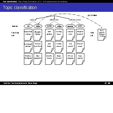
Text classification Naive Bayes Evaluation of TC NB independence assumptions Topic classification γ(d ′) =China regions classes: training set: UK in d u st r i e s China poultry coffee subject areas elections sports c o ngestion O l ympics feed r oasting recount diamo n d London Beijing chicken beans votes baseba l l P a r l iame n t t o urism pate a r a b ica seat f o r wa r d Big Ben Great Wall ducks r o b u s ta r u n -o f f soccer Windsor Mao bird f l u Kenya TV ads team t h e Queen c o mmu n i s t turkey h a rv e s t c a m pa i g n capt ain Schu¨tze: Text classification & Naive Bayes d′ test set: first pr i v a t e C h i n e se a i r l ine 9 / 48

Text classification Naive Bayes Evaluation of TC NB independence assumptions Many search engine functionalities are based on classification. Examples? Schu¨tze: Text classification & Naive Bayes 10 / 48

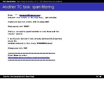
Text classification Naive Bayes Evaluation of TC NB independence assumptions Another TC task: spam filtering From: ‘‘’’ <takworlld@hotmail. com> S u b j e c t : r e a l e s t a t e i s t h e only w a y. . . gem oalvgkay Anyone can buy r e a l e s t a t e with no money down Stop paying r e n t TODAY! There i s no need t o spend hundreds o r even thousands f o r similar courses I am 22 y e a r s o l d and I have a l r e a d y purchased 6 p r o p e r t i e s using the methods o u t l i n e d i n t h i s t r u l y INCREDIBLE ebook. Change your l i f e NOW! ========================= C l i c k Below t o o r d e r : http: //www. wholesaledaily. com/sales/nmd. htm ========================= Schu¨tze: Text classification & Naive Bayes 6 / 48

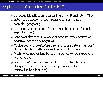
Text classification Naive Bayes Evaluation of TC NB independence assumptions Applications of text classification in IR Language identification (classes: English vs. French etc. ) The automatic detection of spam pages (spam vs. nonspam, example: googel. org) The automatic detection of sexually explicit content (sexually explicit vs. not) Sentiment detection: is a movie or product review positive or negative (positive vs. negative) Topic-specific or vertical search – restrict search to a “vertical” like “related to health” (relevant to vertical vs. not) Machine-learned ranking function in ad hoc retrieval (relevant vs. nonrelevant) Semantic Web: Automatically add semantic tags for non -tagged text (e. g. , for each paragraph: relevant to a vertical like health or not) Schu¨tze: Text classification & Naive Bayes 11 / 48

Text classification Naive Bayes Evaluation of TC NB independence assumptions Outline 1 Text classification 2 Naive Bayes 3 Evaluation of TC 4 NB independence assumptions Schu¨tze: Text classification & Naive Bayes 16 / 48

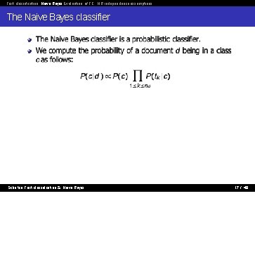
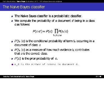
Text classification Naive Bayes Evaluation of TC NB independence assumptions The Naive Bayes classifier Schu¨tze: Text classification & Naive Bayes 17 / 48

Text classification Naive Bayes Evaluation of TC NB independence assumptions The Naive Bayes classifier Schu¨tze: Text classification & Naive Bayes 17 / 48

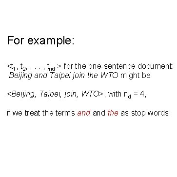
For example: <t 1, t 2, . . . , tnd > for the one-sentence document: Beijing and Taipei join the WTO might be <Beijing, Taipei, join, WTO>, with nd = 4, if we treat the terms and the as stop words

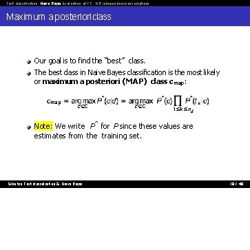
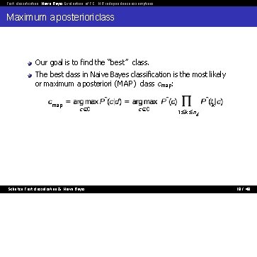
Text classification Naive Bayes Evaluation of TC NB independence assumptions Maximum a posteriori class Our goal is to find the “best” class. The best class in Naive Bayes classification is the most likely or maximum a posteriori (MAP) class cmap: map c∈C 1≤k≤nd Note: We write Pˆ for P since these values are estimates from the training set. Schu¨tze: Text classification & Naive Bayes 18 / 48

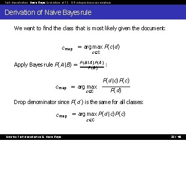
Text classification Naive Bayes Evaluation of TC NB independence assumptions Derivation of Naive Bayesrule We want to find the class that is most likely given the document: cmap = arg max P(c|d ) c∈C Apply Bayes rule P(A|B) = P(B| A)P(A) P (B) cmap = arg max c∈C : P(d |c)P(c) P(d ) Drop denominator since P(d ) is the same for all classes: cmap = arg max P(d |c)P(c) c∈C Schu¨tze: Text classification & Naive Bayes 32 / 48

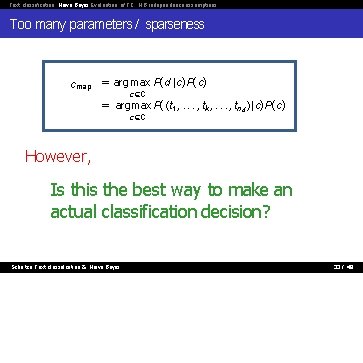
Text classification Naive Bayes Evaluation of TC NB independence assumptions Too many parameters / sparseness cmap = arg max P(d |c)P(c) c∈C = arg max P((t 1 , . . . , tk , . . . , tnd )|c)P(c) c∈C However, Is this the best way to make an actual classification decision? Schu¨tze: Text classification & Naive Bayes 33 / 48

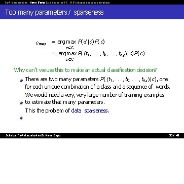
Text classification Naive Bayes Evaluation of TC NB independence assumptions Too many parameters / sparseness cmap = arg max P(d |c)P(c) c∈C = arg max P((t 1 , . . . , tk , . . . , tnd )|c)P(c) c∈C Why can’t we use this to make an actual classification decision? There are two many parameters P((t 1 , . . . , tk , . . . , tnd )|c), one for each unique combination of a class and a sequence of words. We would need a very, very large number of training examples to estimate that many parameters. This the problem of data sparseness. Schu¨tze: Text classification & Naive Bayes 33 / 48

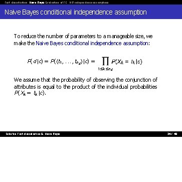
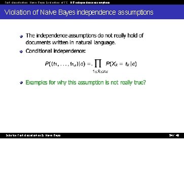
Text classification Naive Bayes Evaluation of TC NB independence assumptions Naive Bayes conditional independence assumption To reduce the number of parameters to a manageable size, we make the Naive Bayes conditional independence assumption: P(d |c) = P((t 1 , . . . , tnd )|c) = 1≤k≤nd We assume that the probability of observing the conjunction of attributes is equal to the product of the individual probabilities P(Xk = tk |c). Recall from earlier the estimates for these priors and conditional probabilities: Pˆ(c) = Nc and Pˆ(t|c) = P Tct + 1 N Schu¨tze: Text classification & Naive Bayes ( t ′∈ V T ct ′ ) + B 34 / 48

Text classification Naive Bayes Evaluation of TC NB independence assumptions Maximum a posteriori class Our goal is to find the “best” class. The best class in Naive Bayes classification is the most likely or maximum a posteriori (MAP) class cmap: map c∈C Schu¨tze: Text classification & Naive Bayes c∈C k 1≤k≤nd 18 / 48

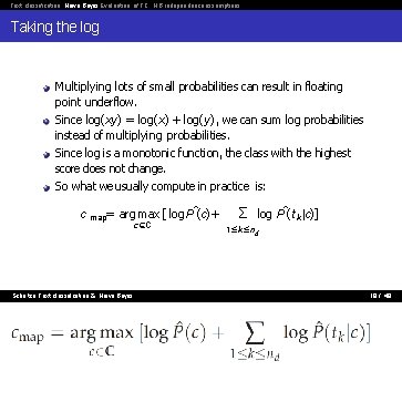
Text classification Naive Bayes Evaluation of TC NB independence assumptions Taking the log Multiplying lots of small probabilities can result in floating point underflow. Since log(xy ) = log(x ) + log(y ), we can sum log probabilities instead of multiplying probabilities. Since log is a monotonic function, the class with the highest score does not change. So what we usually compute in practice is: c map= arg max [ log Pˆ(c) + Schu¨tze: Text classification & Naive Bayes c∈C Σ log Pˆ(t. k|c)] 1≤k≤nd 19 / 48

Text classification Naive Bayes Evaluation of TC NB independence assumptions Parameter estimation How to estimate parameters Pˆ(c) and Pˆ(tk|c) from training data? Schu¨tze: Text classification & Naive Bayes 21 / 48

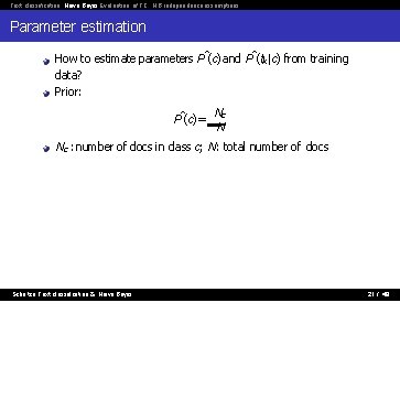
Text classification Naive Bayes Evaluation of TC NB independence assumptions Parameter estimation How to estimate parameters Pˆ(c) and Pˆ(tk|c) from training data? Prior: N Pˆ(c) = c N Nc : number of docs in class c; N: total number of docs Schu¨tze: Text classification & Naive Bayes 21 / 48

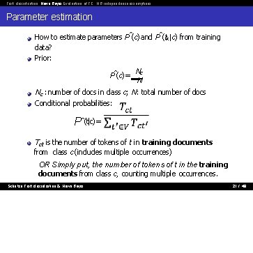
Text classification Naive Bayes Evaluation of TC NB independence assumptions Parameter estimation How to estimate parameters Pˆ(c) and Pˆ(tk|c) from training data? Prior: N Pˆ(c) = c N Nc : number of docs in class c; N: total number of docs Conditional probabilities: Pˆ(t|c) = Tct is the number of tokens of t in training documents from class c (includes multiple occurrences) OR Simply put, the number of tokens of t in the training documents from class c, counting multiple occurrences. Schu¨tze: Text classification & Naive Bayes 21 / 48

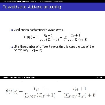
Text classification Naive Bayes Evaluation of TC NB independence assumptions To avoid zeros: Add-one smoothing Add one to each count to avoid zeros: Pˆ(t|c) = Σ Tct + 1 = Σ ( t′∈V (Tct′ + 1) Tct + 1 t′∈V T ct ′ ) + B B is the number of different words (in this case the size of the vocabulary: |V | = M) Schu¨tze: Text classification & Naive Bayes 23 / 48

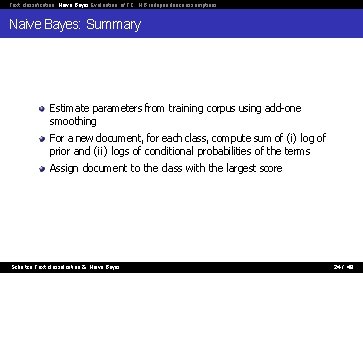
Text classification Naive Bayes Evaluation of TC NB independence assumptions Naive Bayes: Summary Estimate parameters from training corpus using add-one smoothing For a new document, for each class, compute sum of (i) log of prior and (ii) logs of conditional probabilities of the terms Assign document to the class with the largest score Schu¨tze: Text classification & Naive Bayes 24 / 48

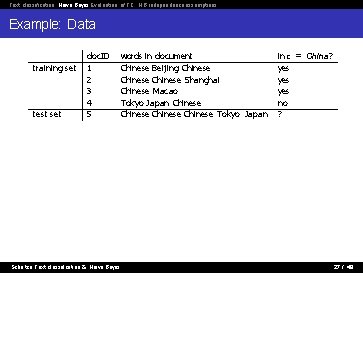
Text classification Naive Bayes Evaluation of TC NB independence assumptions Example: Data training set test set doc. ID 1 2 3 4 5 Schu¨tze: Text classification & Naive Bayes words in document Chinese Beijing Chinese Shanghai Chinese Macao Tokyo Japan Chinese Tokyo Japan in c = China? yes yes no ? 27 / 48

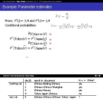
Text classification Naive Bayes Evaluation of TC NB independence assumptions Example: Parameter estimates Priors: Pˆ(c) = 3/4 and Pˆ(c) = 1/4 Conditional probabilities: ˆ (C h in e se |c) P Pˆ (Tokyo|c) = Pˆ(Japan|c) = = Schu¨tze: Text classification & Naive Bayes training set test set doc. ID 1 2 3 4 5 28 / 48 words in document Chinese Beijing Chinese Shanghai Chinese Macao Tokyo Japan Chinese Tokyo Japan in c = China? yes yes no ?

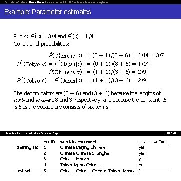
Text classification Naive Bayes Evaluation of TC NB independence assumptions Example: Parameter estimates Priors: Pˆ(c) = 3/4 and Pˆ(c) = 1/4 Conditional probabilities: ˆ (C h in e se |c) = (5 + P Pˆ (Tokyo|c) = Pˆ(Japan|c) = (0 + ˆ (C h in e se |c) = (1 + P Pˆ (Tokyo|c) = Pˆ(Japan|c) = (1 + 1)/(8 + 6) = 6/14 = 3/7 1)/(8 + 6) = 1/14 1)/(3 + 6) = 2/9 The denominators are (8 + 6) and (3 + 6) because the lengths of textc and textc are 8 and 3, respectively, and because the constant B is 6 as the vocabulary consists of six terms. Schu¨tze: Text classification & Naive Bayes training set test set doc. ID 1 2 3 4 5 28 / 48 words in document Chinese Beijing Chinese Shanghai Chinese Macao Tokyo Japan Chinese Tokyo Japan in c = China? yes yes no ?

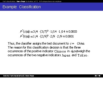
Text classification Naive Bayes Evaluation of TC NB independence assumptions Example: Classification Pˆ(c|d 5) ∝ 3/4 ·(3/7)3 · 1/14 ≈ 0. 0003 Pˆ(c|d 5) ∝ 1/4 ·(2/9)3 · 2/9 ≈ 0. 0001 Thus, the classifier assigns the test document to c = China. The reason for this classification decision is that the three occurrences of the positive indicator C h i n e s e in d 5 outweigh the occurrences of the two negative indicators J a p a n and T o k y o. Schu¨tze: Text classification & Naive Bayes 29 / 48

Text classification Naive Bayes Evaluation of TC NB independence assumptions Outline 1 Text classification 2 Naive Bayes 3 Evaluation of TC 4 NB independence assumptions Schu¨tze: Text classification & Naive Bayes 44 / 48

Text classification Naive Bayes Evaluation of TC NB independence assumptions Violation of Naive Bayes independence assumptions Schu¨tze: Text classification & Naive Bayes 54 / 48

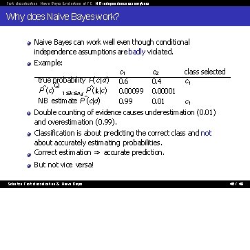
Text classification Naive Bayes Evaluation of TC NB independence assumptions Why does Naive Bayes work? Naive Bayes can work well even though conditional independence assumptions are badly violated. Example: c 1 c 2 class selected true probability P(c|d ) 0. 6 c 1 0. 4 Q Pˆ(c) 1≤k≤nd Pˆ(tk|c) 0. 00099 0. 00001 NB estimate Pˆ(c|d) c 1 0. 99 0. 01 Schu¨tze: Text classification & Naive Bayes 46 / 48

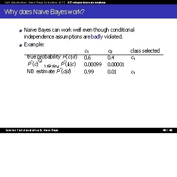
Text classification Naive Bayes Evaluation of TC NB independence assumptions Why does Naive Bayes work? Naive Bayes can work well even though conditional independence assumptions are badly violated. Example: c 1 c 2 class selected true probability P(c|d ) 0. 6 c 1 0. 4 Q Pˆ(c) 1≤k≤nd Pˆ(tk|c) 0. 00099 0. 00001 NB estimate Pˆ(c|d) c 1 0. 99 0. 01 Double counting of evidence causes underestimation (0. 01) and overestimation (0. 99). Classification is about predicting the correct class and not about accurately estimating probabilities. Correct estimation ⇒ accurate prediction. But not vice versa! Schu¨tze: Text classification & Naive Bayes 46 / 48

Text classification Naive Bayes Evaluation of TC NB independence assumptions Naive Bayes is not so naive Naive Bayes has won some bakeoffs (e. g. , KDD-CUP 97) More robust to nonrelevant features than some more complex learning methods More robust to concept drift (changing of definition of class over time) than some more complex learning methods Better than methods like decision trees when we have many equally important features A good dependable baseline for text classification (but not the best) Optimal if independence assumptions hold (never true for text, but true for some domains) Very fast Low storage requirements Schu¨tze: Text classification & Naive Bayes 47 / 48