Vector Spaces 1 Vectors in Rn 2 Vector

Vector Spaces 1. Vectors in Rn 2. Vector Spaces 3. Subspaces of Vector Spaces 4. Spanning Sets and Linear Independence 5. Basis and Dimension 6. Rank of a Matrix and Systems of Linear Equations 7. Coordinates and Change of Basis 8. Applications of Vector Spaces 4.

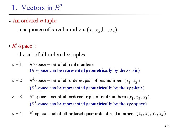
1. Vectors in R n n An ordered n-tuple: a sequence of n real numbers n § R -space : the set of all ordered n-tuples n = 1 R 1 -space = set of all real numbers (R 1 -space can be represented geometrically by the x-axis) n = 2 R 2 -space = set of all ordered pair of real numbers (R 2 -space can be represented geometrically by the xy-plane) n = 3 R 3 -space = set of all ordered triple of real numbers (R 3 -space can be represented geometrically by the xyz-space) n = 4 R 4 -space = set of all ordered quadruple of real numbers 4. 2

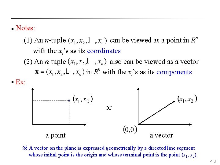
n Notes: (1) An n-tuple can be viewed as a point in Rn with the xi’s as its coordinates (2) An n-tuple also can be viewed as a vector in Rn with the xi’s as its components § Ex: or a point a vector ※ A vector on the plane is expressed geometrically by a directed line segment whose initial point is the origin and whose terminal point is the point (x 1, x 2) 4. 3

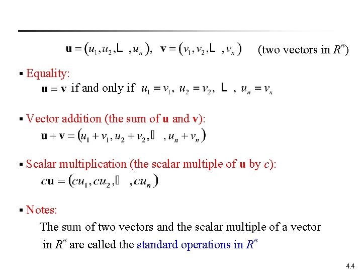
n (two vectors in R ) § Equality: if and only if § Vector addition (the sum of u and v): § Scalar multiplication (the scalar multiple of u by c): § Notes: The sum of two vectors and the scalar multiple of a vector in Rn are called the standard operations in Rn 4. 4

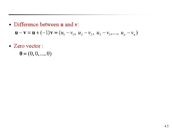
§ Difference between u and v: § Zero vector : 4. 5

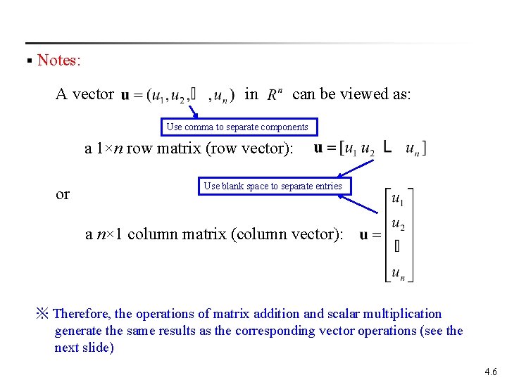
§ Notes: A vector in can be viewed as: Use comma to separate components a 1×n row matrix (row vector): or Use blank space to separate entries a n× 1 column matrix (column vector): ※ Therefore, the operations of matrix addition and scalar multiplication generate the same results as the corresponding vector operations (see the next slide) 4. 6

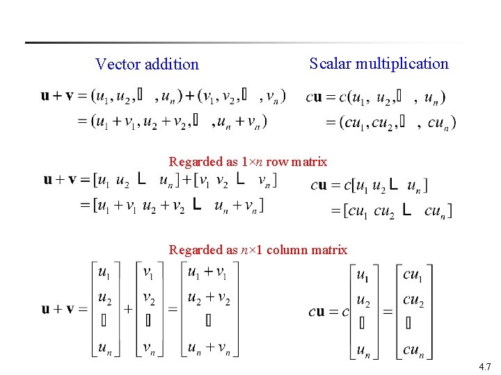
Vector addition Scalar multiplication Regarded as 1×n row matrix Regarded as n× 1 column matrix 4. 7

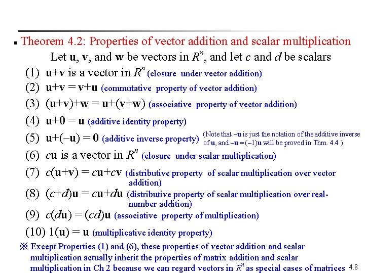
Theorem 4. 2: Properties of vector addition and scalar multiplication Let u, v, and w be vectors in Rn, and let c and d be scalars (1) u+v is a vector in Rn (closure under vector addition) (2) u+v = v+u (commutative property of vector addition) (3) (u+v)+w = u+(v+w) (associative property of vector addition) (4) u+0 = u (additive identity property) (5) u+(–u) = 0 (additive inverse property) (Note that –u is just the notation of the additive inverse of u, and –u = (– 1)u will be proved in Thm. 4. 4 ) (6) cu is a vector in Rn (closure under scalar multiplication) (7) c(u+v) = cu+cv (distributive property of scalar multiplication over vector n addition) (8) (c+d)u = cu+du (distributive property of scalar multiplication over realnumber addition) (9) c(du) = (cd)u (associative property of multiplication) (10) 1(u) = u (multiplicative identity property) ※ Except Properties (1) and (6), these properties of vector addition and scalar multiplication actually inherit the properties of matrix addition and scalar multiplication in Ch 2 because we can regard vectors in Rn as special cases of matrices 4. 8

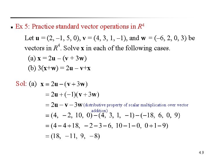
n Ex 5: Practice standard vector operations in R 4 Let u = (2, – 1, 5, 0), v = (4, 3, 1, – 1), and w = (– 6, 2, 0, 3) be vectors in R 4. Solve x in each of the following cases. (a) x = 2 u – (v + 3 w) (b) 3(x+w) = 2 u – v+x Sol: (a) (distributive property of scalar multiplication over vector addition) 4. 9

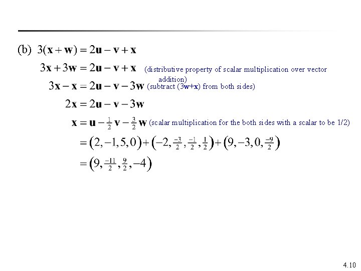
(b) (distributive property of scalar multiplication over vector addition) (subtract (3 w+x) from both sides) (scalar multiplication for the both sides with a scalar to be 1/2) 4. 10

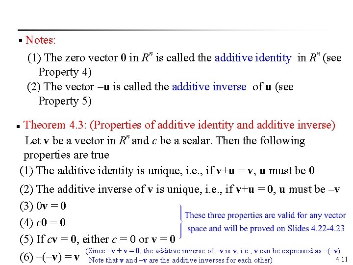
§ Notes: n n (1) The zero vector 0 in R is called the additive identity in R (see Property 4) (2) The vector –u is called the additive inverse of u (see Property 5) Theorem 4. 3: (Properties of additive identity and additive inverse) Let v be a vector in Rn and c be a scalar. Then the following properties are true (1) The additive identity is unique, i. e. , if v+u = v, u must be 0 n (2) The additive inverse of v is unique, i. e. , if v+u = 0, u must be –v (3) 0 v = 0 (4) c 0 = 0 (5) If cv = 0, either c = 0 or v = 0 (Since –v + v = 0, the additive inverse of –v is v, i. e. , v can be expressed as –(–v). (6) –(–v) = v Note that v and –v are the additive inverses for each other) 4. 11

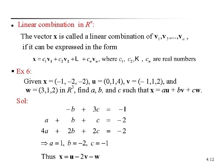
n n Linear combination in R : The vector x is called a linear combination of , if it can be expressed in the form § Ex 6: Given x = (– 1, – 2), u = (0, 1, 4), v = (– 1, 1, 2), and w = (3, 1, 2) in R 3, find a, b, and c such that x = au + bv + cw. Sol: 4. 12

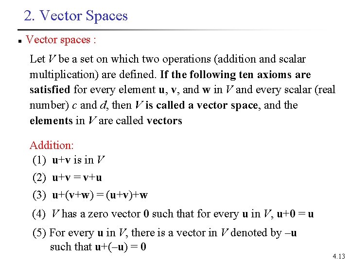
2. Vector Spaces n Vector spaces : Let V be a set on which two operations (addition and scalar multiplication) are defined. If the following ten axioms are satisfied for every element u, v, and w in V and every scalar (real number) c and d, then V is called a vector space, and the elements in V are called vectors Addition: (1) u+v is in V (2) u+v = v+u (3) u+(v+w) = (u+v)+w (4) V has a zero vector 0 such that for every u in V, u+0 = u (5) For every u in V, there is a vector in V denoted by –u such that u+(–u) = 0 4. 13

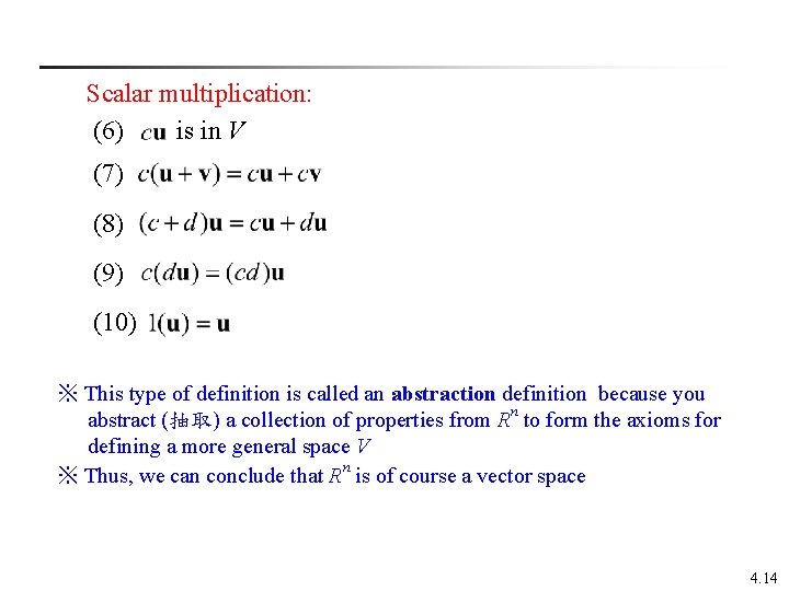
Scalar multiplication: (6) is in V (7) (8) (9) (10) ※ This type of definition is called an abstraction definition because you abstract (抽取) a collection of properties from Rn to form the axioms for defining a more general space V ※ Thus, we can conclude that Rn is of course a vector space 4. 14

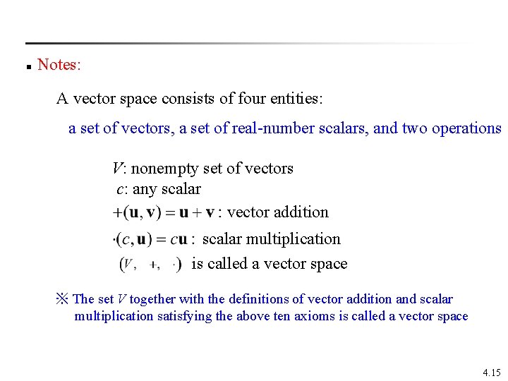
n Notes: A vector space consists of four entities: a set of vectors, a set of real-number scalars, and two operations V: nonempty set of vectors c: any scalar vector addition scalar multiplication is called a vector space ※ The set V together with the definitions of vector addition and scalar multiplication satisfying the above ten axioms is called a vector space 4. 15

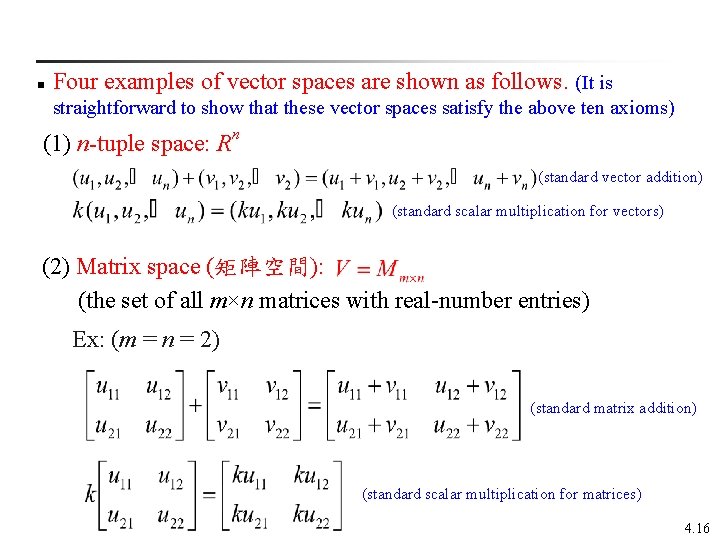
n Four examples of vector spaces are shown as follows. (It is straightforward to show that these vector spaces satisfy the above ten axioms) (1) n-tuple space: Rn (standard vector addition) (standard scalar multiplication for vectors) (2) Matrix space (矩陣空間): (the set of all m×n matrices with real-number entries) Ex: (m = n = 2) (standard matrix addition) (standard scalar multiplication for matrices) 4. 16

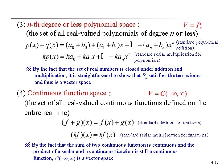
(3) n-th degree or less polynomial space : (the set of all real-valued polynomials of degree n or less) (standard polynomial addition) (standard scalar multiplication for polynomials) ※ By the fact that the set of real numbers is closed under addition and multiplication, it is straightforward to show that Pn satisfies the ten axioms and thus is a vector space (4) Continuous function space : (the set of all real-valued continuous functions defined on the entire real line) (standard addition for functions) (standard scalar multiplication for functions) ※ By the fact that the sum of two continuous function is continuous and the product of a scalar and a continuous function is still a continuous function, is a vector space 4. 17

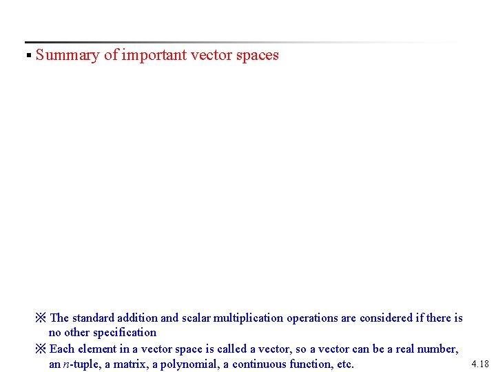
§ Summary of important vector spaces ※ The standard addition and scalar multiplication operations are considered if there is no other specification ※ Each element in a vector space is called a vector, so a vector can be a real number, an n-tuple, a matrix, a polynomial, a continuous function, etc. 4. 18

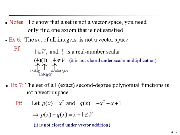
Notes: To show that a set is not a vector space, you need only find one axiom that is not satisfied n Ex 6: The set of all integers is not a vector space Pf: n (it is not closed under scalar multiplication) scalar noninteger Ex 7: The set of all (exact) second-degree polynomial functions is not a vector space n Pf: Let and (it is not closed under vector addition) 4. 19

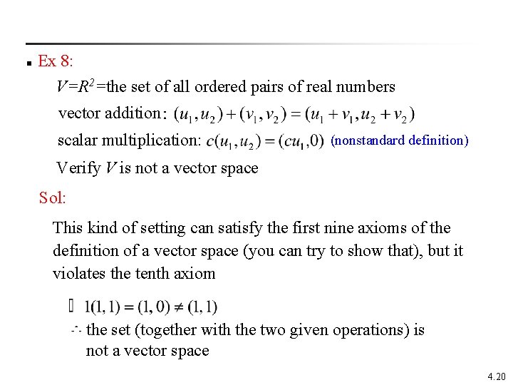
n Ex 8: V=R 2=the set of all ordered pairs of real numbers vector addition: scalar multiplication: (nonstandard definition) Verify V is not a vector space Sol: This kind of setting can satisfy the first nine axioms of the definition of a vector space (you can try to show that), but it violates the tenth axiom the set (together with the two given operations) is not a vector space 4. 20

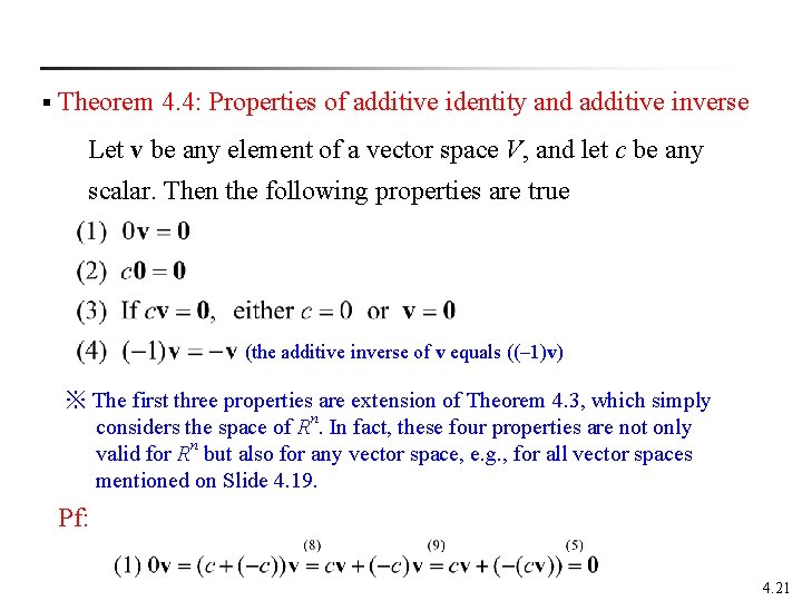
§ Theorem 4. 4: Properties of additive identity and additive inverse Let v be any element of a vector space V, and let c be any scalar. Then the following properties are true (the additive inverse of v equals ((– 1)v) ※ The first three properties are extension of Theorem 4. 3, which simply considers the space of Rn. In fact, these four properties are not only valid for Rn but also for any vector space, e. g. , for all vector spaces mentioned on Slide 4. 19. Pf: 4. 21

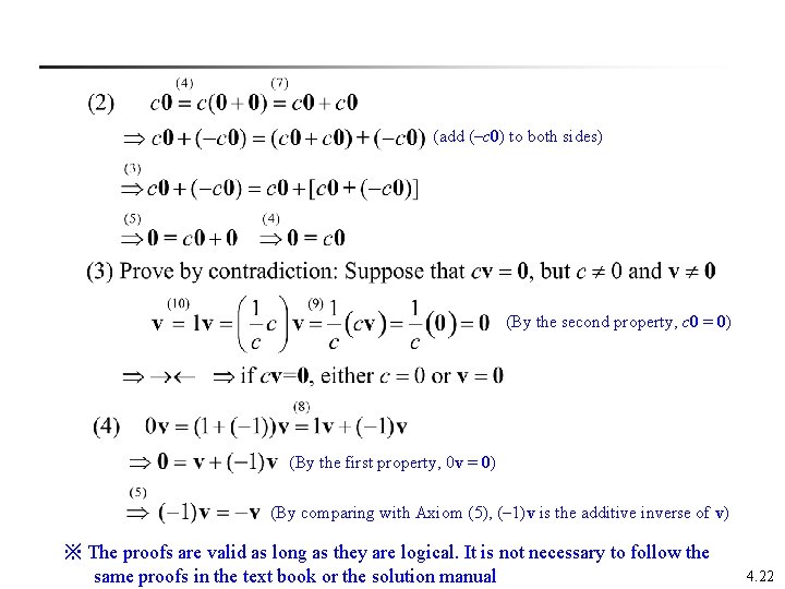
(add (–c 0) to both sides) (By the second property, c 0 = 0) (By the first property, 0 v = 0) (By comparing with Axiom (5), (– 1)v is the additive inverse of v) ※ The proofs are valid as long as they are logical. It is not necessary to follow the same proofs in the text book or the solution manual 4. 22

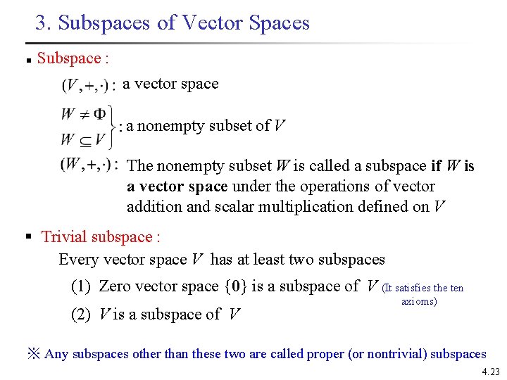
3. Subspaces of Vector Spaces n Subspace : a vector space a nonempty subset of V The nonempty subset W is called a subspace if W is a vector space under the operations of vector addition and scalar multiplication defined on V § Trivial subspace : Every vector space V has at least two subspaces (1) Zero vector space {0} is a subspace of V (It satisfies the ten (2) V is a subspace of V axioms) ※ Any subspaces other than these two are called proper (or nontrivial) subspaces 4. 23

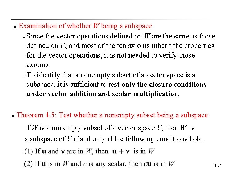
n n Examination of whether W being a subspace – Since the vector operations defined on W are the same as those defined on V, and most of the ten axioms inherit the properties for the vector operations, it is not needed to verify those axioms – To identify that a nonempty subset of a vector space is a subspace, it is sufficient to test only the closure conditions under vector addition and scalar multiplication. Theorem 4. 5: Test whether a nonempty subset being a subspace If W is a nonempty subset of a vector space V, then W is a subspace of V if and only if the following conditions hold 4. 24

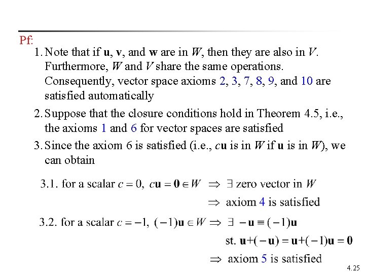
Pf: 1. Note that if u, v, and w are in W, then they are also in V. Furthermore, W and V share the same operations. Consequently, vector space axioms 2, 3, 7, 8, 9, and 10 are satisfied automatically 2. Suppose that the closure conditions hold in Theorem 4. 5, i. e. , the axioms 1 and 6 for vector spaces are satisfied 3. Since the axiom 6 is satisfied (i. e. , cu is in W if u is in W), we can obtain 4. 25

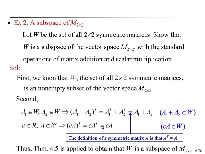
§ Ex 2: A subspace of M 2× 2 Let W be the set of all 2× 2 symmetric matrices. Show that W is a subspace of the vector space M 2× 2, with the standard operations of matrix addition and scalar multiplication Sol: The definition of a symmetric matrix A is that AT = A 4. 26

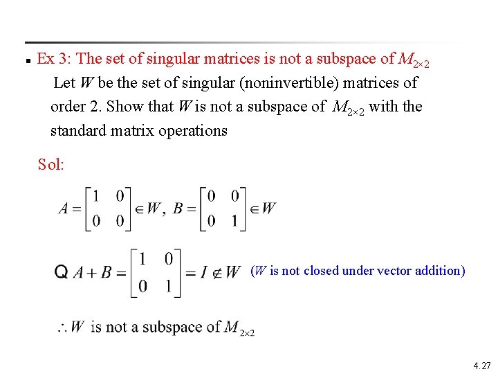
Ex 3: The set of singular matrices is not a subspace of M 2× 2 Let W be the set of singular (noninvertible) matrices of order 2. Show that W is not a subspace of M 2× 2 with the standard matrix operations n Sol: (W is not closed under vector addition) 4. 27

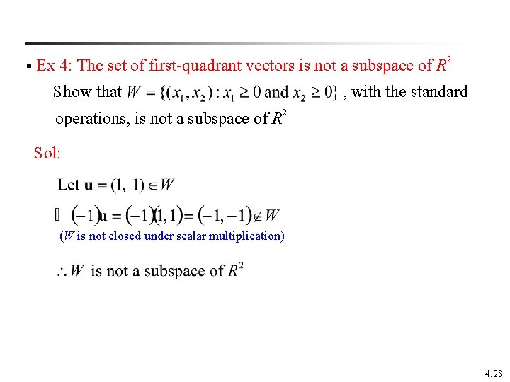
§ Ex 4: The set of first-quadrant vectors is not a subspace of R 2 Show that , with the standard operations, is not a subspace of R 2 Sol: (W is not closed under scalar multiplication) 4. 28

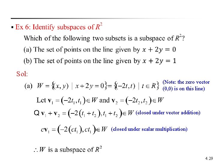
Sol: (Note: the zero vector (0, 0) is on this line) (closed under vector addition) (closed under scalar multiplication) 4. 29

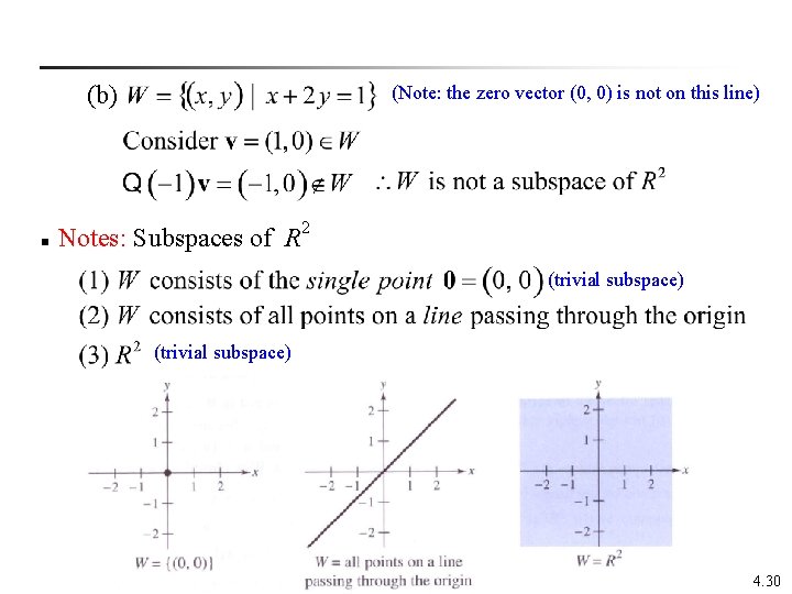
(b) n (Note: the zero vector (0, 0) is not on this line) Notes: Subspaces of R 2 (trivial subspace) 4. 30

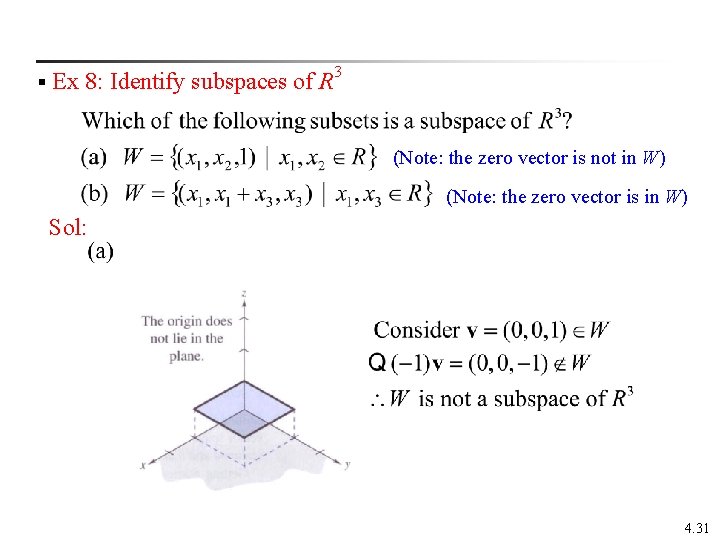
§ Ex 8: Identify subspaces of R 3 (Note: the zero vector is not in W) (Note: the zero vector is in W) Sol: 4. 31

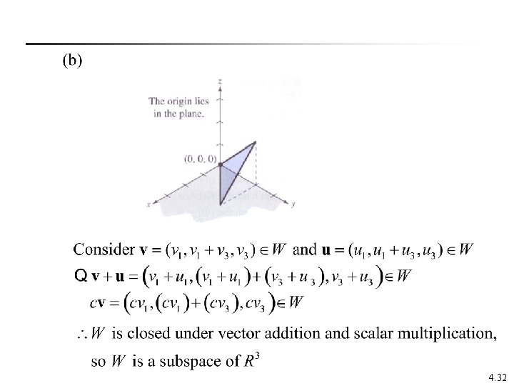
4. 32

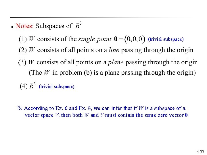
n Notes: Subspaces of R 3 (trivial subspace) ※ According to Ex. 6 and Ex. 8, we can infer that if W is a subspace of a vector space V, then both W and V must contain the same zero vector 0 4. 33

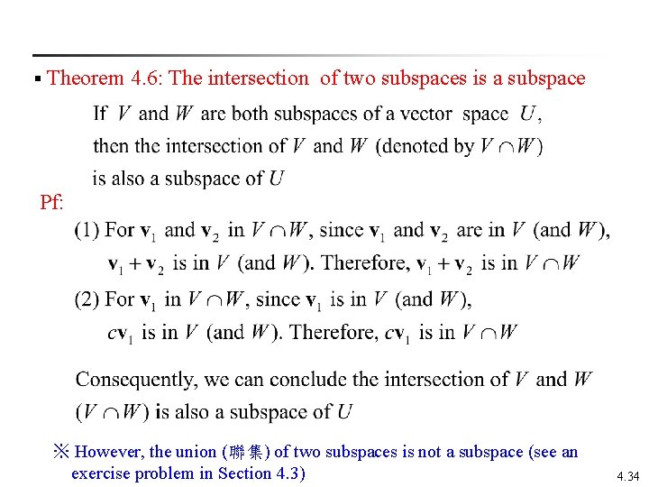
§ Theorem 4. 6: The intersection of two subspaces is a subspace Pf: ※ However, the union (聯集) of two subspaces is not a subspace (see an exercise problem in Section 4. 3) 4. 34

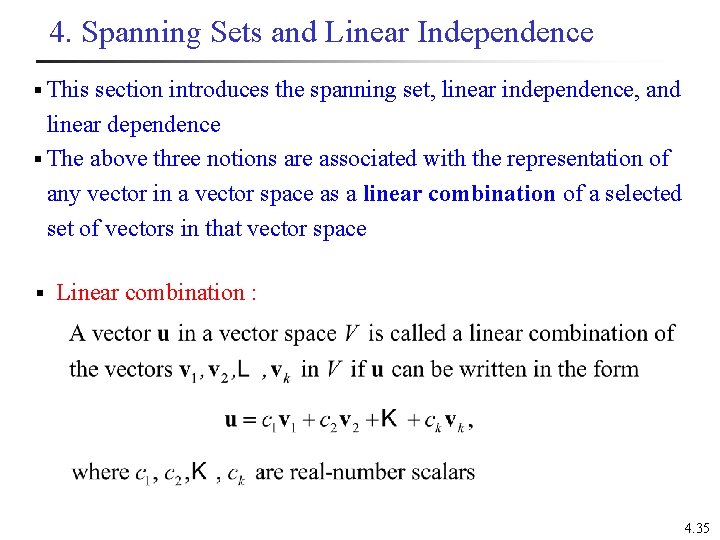
4. Spanning Sets and Linear Independence § This section introduces the spanning set, linear independence, and linear dependence § The above three notions are associated with the representation of any vector in a vector space as a linear combination of a selected set of vectors in that vector space § Linear combination : 4. 35

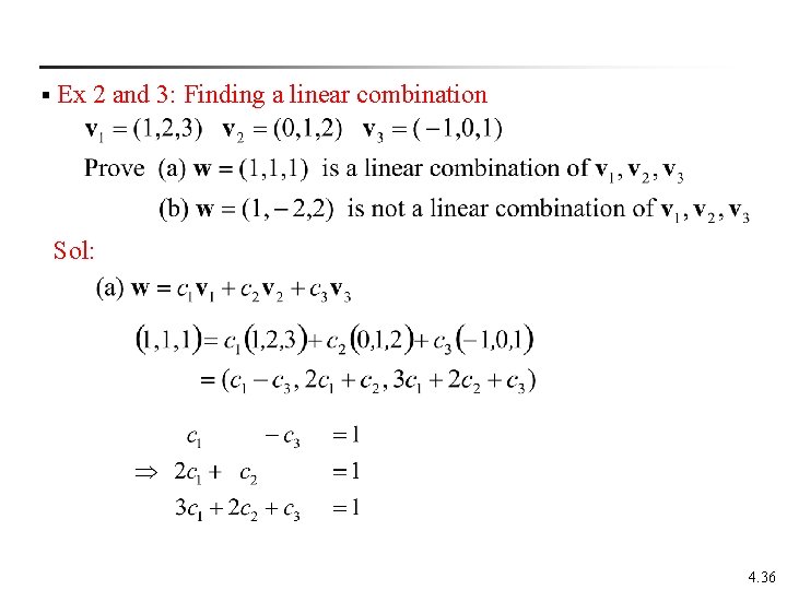
§ Ex 2 and 3: Finding a linear combination Sol: 4. 36

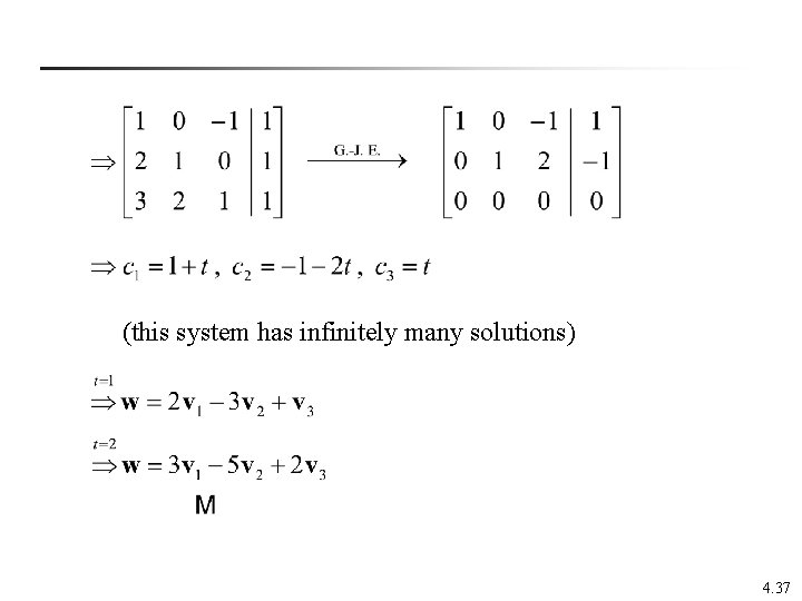
(this system has infinitely many solutions) 4. 37

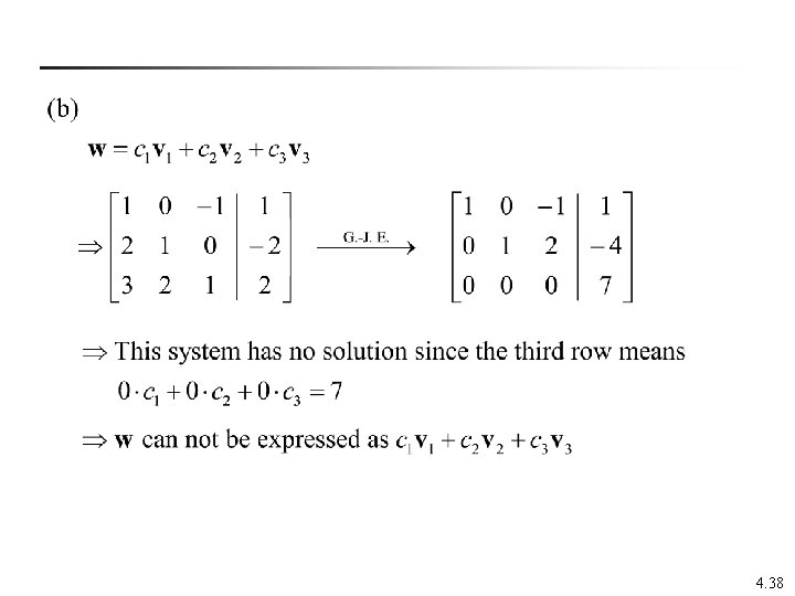
4. 38

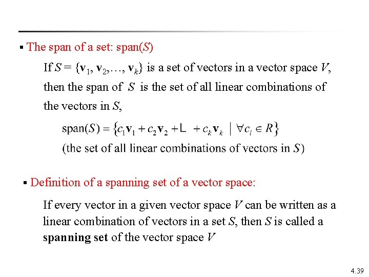
§ The span of a set: span(S) If S = {v 1, v 2, …, vk} is a set of vectors in a vector space V, then the span of S is the set of all linear combinations of the vectors in S, § Definition of a spanning set of a vector space: If every vector in a given vector space V can be written as a linear combination of vectors in a set S, then S is called a spanning set of the vector space V 4. 39

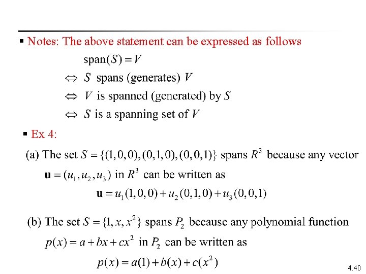
§ Notes: The above statement can be expressed as follows § Ex 4: 4. 40

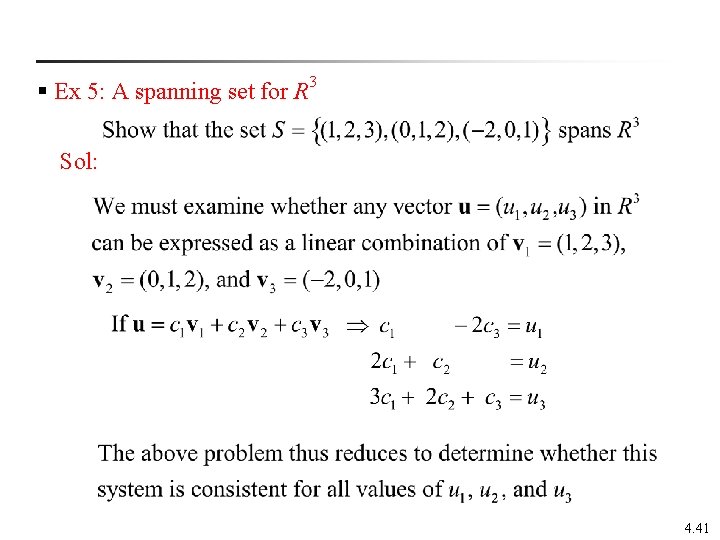
§ Ex 5: A spanning set for R 3 Sol: 4. 41

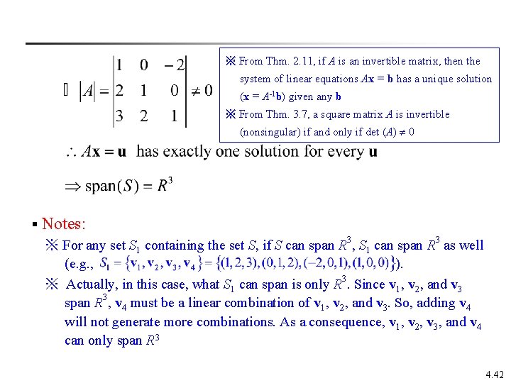
※ From Thm. 2. 11, if A is an invertible matrix, then the system of linear equations Ax = b has a unique solution (x = A-1 b) given any b ※ From Thm. 3. 7, a square matrix A is invertible (nonsingular) if and only if det (A) 0 § Notes: ※ For any set S 1 containing the set S, if S can span R 3, S 1 can span R 3 as well (e. g. , ). ※ Actually, in this case, what S 1 can span is only R 3. Since v 1, v 2, and v 3 span R 3, v 4 must be a linear combination of v 1, v 2, and v 3. So, adding v 4 will not generate more combinations. As a consequence, v 1, v 2, v 3, and v 4 can only span R 3 4. 42

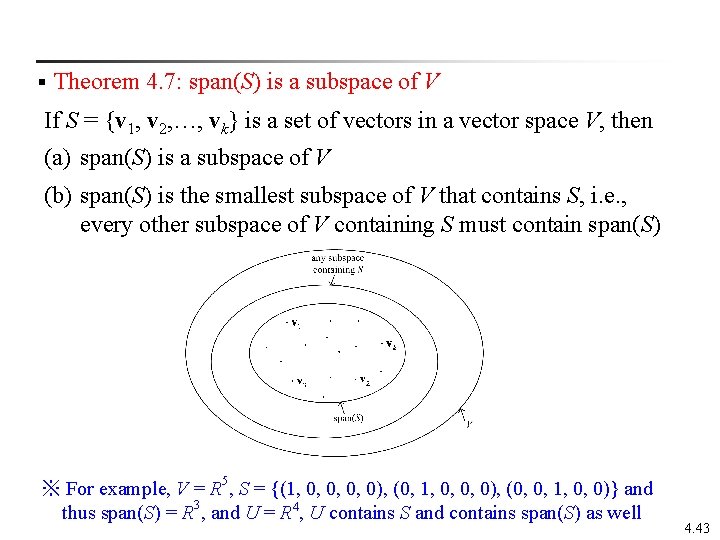
§ Theorem 4. 7: span(S) is a subspace of V If S = {v 1, v 2, …, vk} is a set of vectors in a vector space V, then (a) span(S) is a subspace of V (b) span(S) is the smallest subspace of V that contains S, i. e. , every other subspace of V containing S must contain span(S) ※ For example, V = R 5, S = {(1, 0, 0), (0, 1, 0, 0, 0), (0, 0, 1, 0, 0)} and thus span(S) = R 3, and U = R 4, U contains S and contains span(S) as well 4. 43

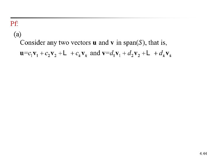
Pf: (a) 4. 44

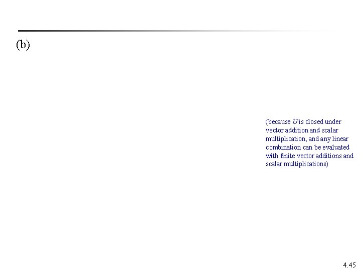
(b) (because U is closed under vector addition and scalar multiplication, and any linear combination can be evaluated with finite vector additions and scalar multiplications) 4. 45

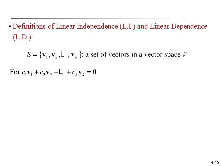
§ Definitions of Linear Independence (L. I. ) and Linear Dependence (L. D. ) : 4. 46

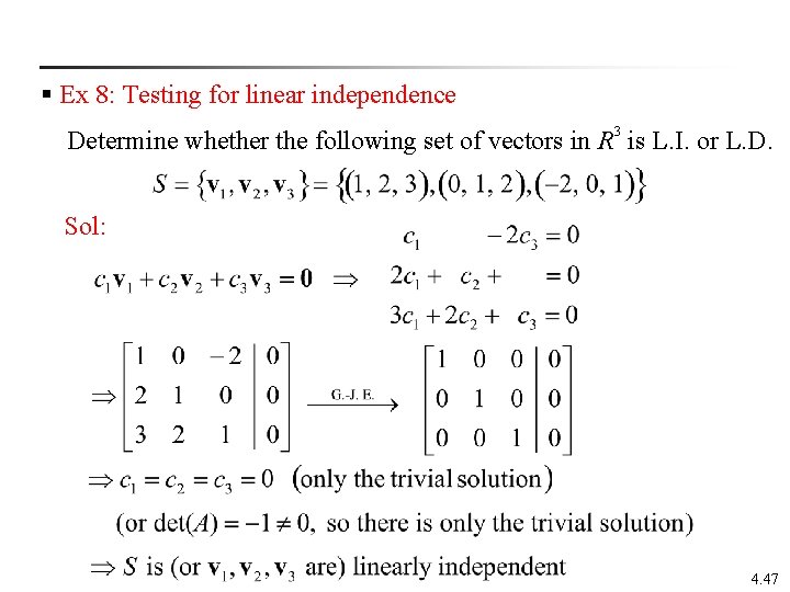
§ Ex 8: Testing for linear independence 3 Determine whether the following set of vectors in R is L. I. or L. D. Sol: 4. 47

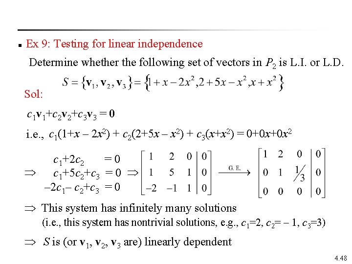
n Ex 9: Testing for linear independence Determine whether the following set of vectors in P 2 is L. I. or L. D. Sol: c 1 v 1+c 2 v 2+c 3 v 3 = 0 i. e. , c 1(1+x – 2 x 2) + c 2(2+5 x – x 2) + c 3(x+x 2) = 0+0 x+0 x 2 c 1+2 c 2 = 0 c 1+5 c 2+c 3 = 0 – 2 c 1– c 2+c 3 = 0 This system has infinitely many solutions (i. e. , this system has nontrivial solutions, e. g. , c 1=2, c 2= – 1, c 3=3) S is (or v 1, v 2, v 3 are) linearly dependent 4. 48

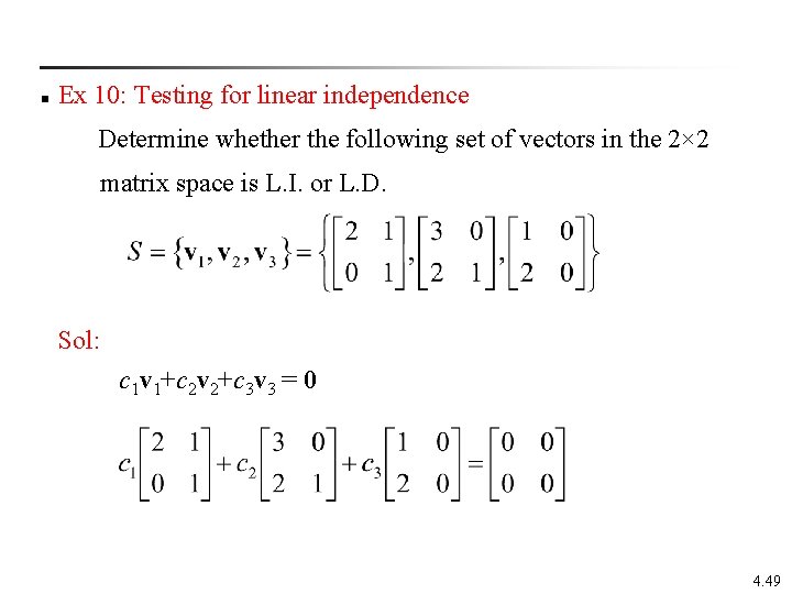
n Ex 10: Testing for linear independence Determine whether the following set of vectors in the 2× 2 matrix space is L. I. or L. D. Sol: c 1 v 1+c 2 v 2+c 3 v 3 = 0 4. 49

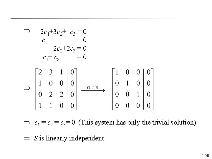
2 c 1+3 c 2+ c 3 = 0 c 1 = 0 2 c 2+2 c 3 = 0 c 1+ c 2 = 0 c 1 = c 2 = c 3= 0 (This system has only the trivial solution) S is linearly independent 4. 50

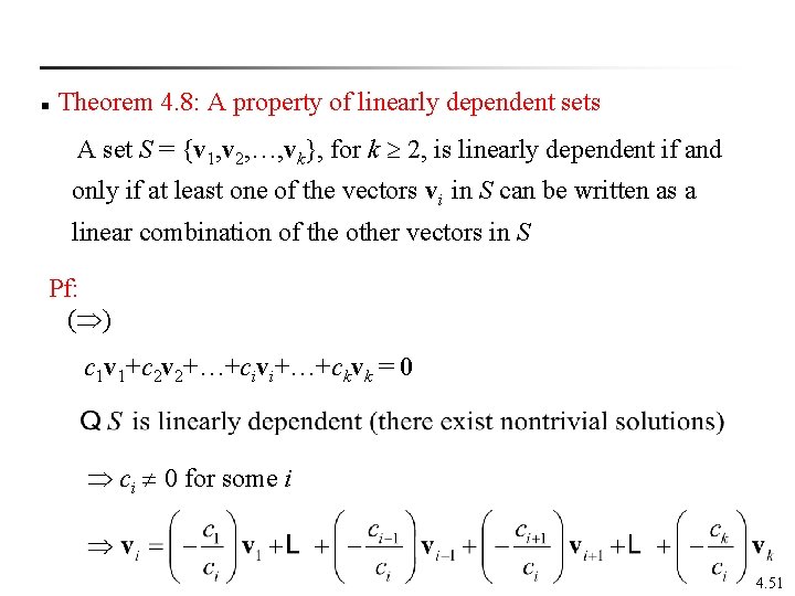
n Theorem 4. 8: A property of linearly dependent sets A set S = {v 1, v 2, …, vk}, for k 2, is linearly dependent if and only if at least one of the vectors vi in S can be written as a linear combination of the other vectors in S Pf: ( ) c 1 v 1+c 2 v 2+…+civi+…+ckvk = 0 ci 0 for some i 4. 51

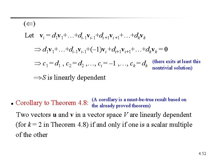
Let vi = d 1 v 1+…+di-1 vi-1+di+1 vi+1+…+dkvk d 1 v 1+…+di-1 vi-1+(– 1)vi +di+1 vi+1+…+dkvk = 0 c 1 = d 1 , c 2 = d 2 , …, ci = – 1 , …, ck = dk (there exits at least this nontrivial solution) S is linearly dependent n Corollary to Theorem 4. 8: (A corollary is a must-be-true result based on the already proved theorem) Two vectors u and v in a vector space V are linearly dependent (for k = 2 in Theorem 4. 8) if and only if one is a scalar multiple of the other 4. 52

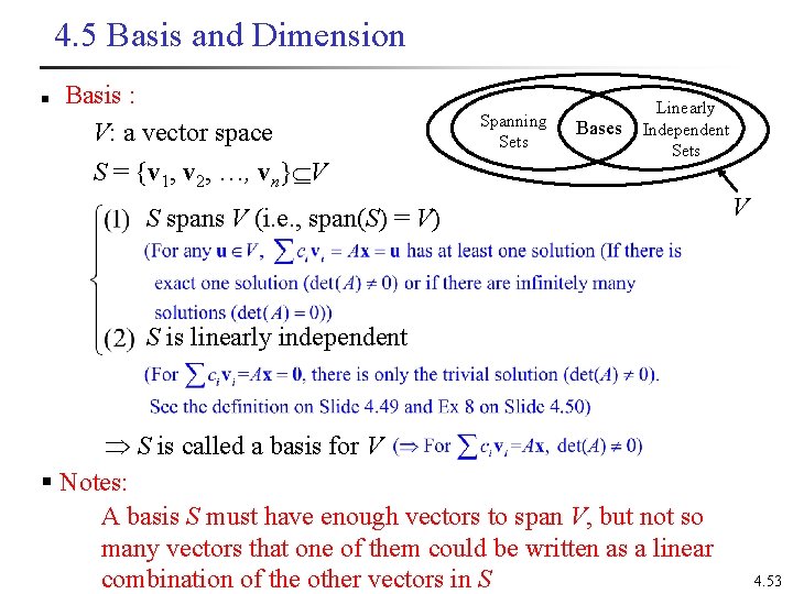
4. 5 Basis and Dimension n Basis : V: a vector space S = {v 1, v 2, …, vn} V Spanning Sets Bases Linearly Independent Sets S spans V (i. e. , span(S) = V) V S is linearly independent S is called a basis for V § Notes: A basis S must have enough vectors to span V, but not so many vectors that one of them could be written as a linear combination of the other vectors in S 4. 53

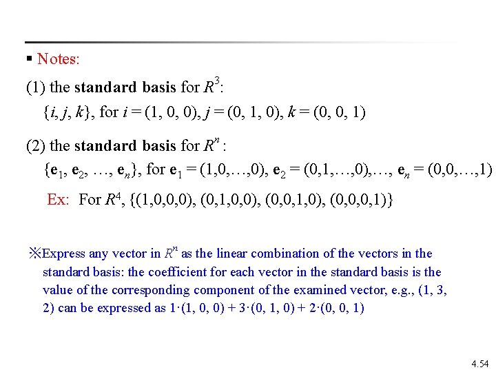
§ Notes: 3 (1) the standard basis for R : {i, j, k}, for i = (1, 0, 0), j = (0, 1, 0), k = (0, 0, 1) (2) the standard basis for Rn : {e 1, e 2, …, en}, for e 1 = (1, 0, …, 0), e 2 = (0, 1, …, 0), …, en = (0, 0, …, 1) Ex: For R 4, {(1, 0, 0, 0), (0, 1, 0, 0), (0, 0, 1, 0), (0, 0, 0, 1)} ※Express any vector in Rn as the linear combination of the vectors in the standard basis: the coefficient for each vector in the standard basis is the value of the corresponding component of the examined vector, e. g. , (1, 3, 2) can be expressed as 1·(1, 0, 0) + 3·(0, 1, 0) + 2·(0, 0, 1) 4. 54

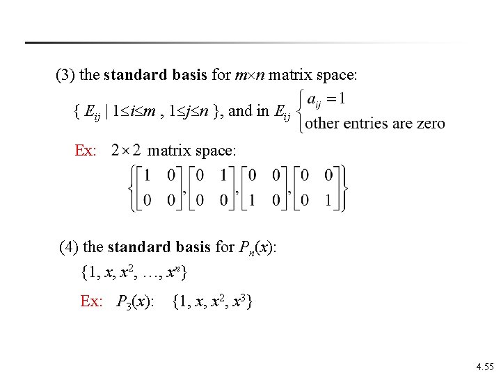
(3) the standard basis for m n matrix space: { Eij | 1 i m , 1 j n }, and in Eij Ex: matrix space: (4) the standard basis for Pn(x): {1, x, x 2, …, xn} Ex: P 3(x): {1, x, x 2, x 3} 4. 55

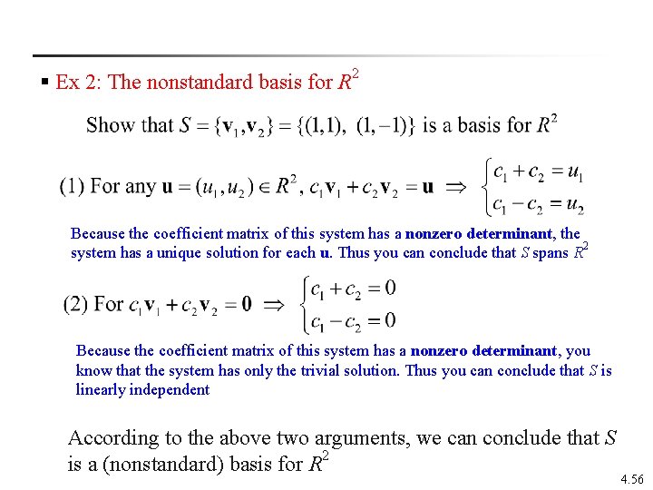
§ Ex 2: The nonstandard basis for R 2 Because the coefficient matrix of this system has a nonzero determinant, the system has a unique solution for each u. Thus you can conclude that S spans R 2 Because the coefficient matrix of this system has a nonzero determinant, you know that the system has only the trivial solution. Thus you can conclude that S is linearly independent According to the above two arguments, we can conclude that S is a (nonstandard) basis for R 2 4. 56

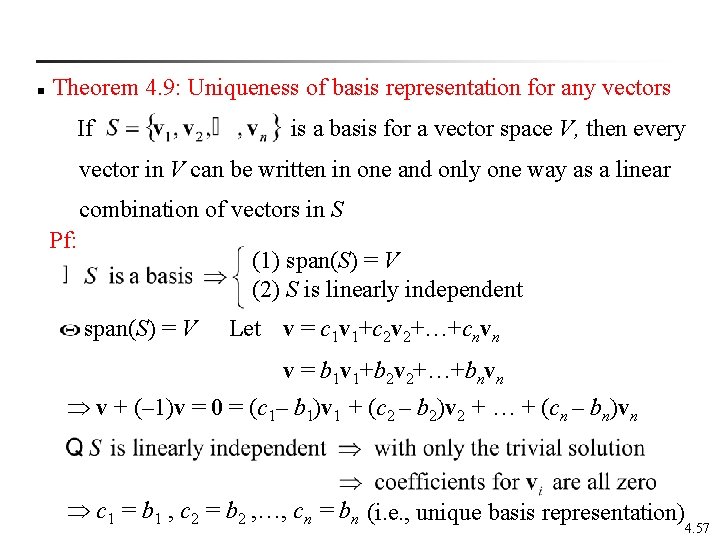
n Theorem 4. 9: Uniqueness of basis representation for any vectors If is a basis for a vector space V, then every vector in V can be written in one and only one way as a linear combination of vectors in S Pf: (1) span(S) = V (2) S is linearly independent span(S) = V Let v = c 1 v 1+c 2 v 2+…+cnvn v = b 1 v 1+b 2 v 2+…+bnvn v + (– 1)v = 0 = (c 1– b 1)v 1 + (c 2 – b 2)v 2 + … + (cn – bn)vn c 1 = b 1 , c 2 = b 2 , …, cn = bn (i. e. , unique basis representation) 4. 57

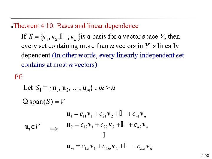
Theorem 4. 10: Bases and linear dependence n If is a basis for a vector space V, then every set containing more than n vectors in V is linearly dependent (In other words, every linearly independent set contains at most n vectors) Pf: Let S 1 = {u 1, u 2, …, um} , m > n ui V 4. 58

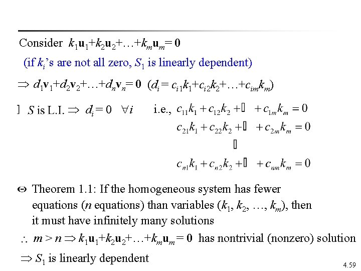
Consider k 1 u 1+k 2 u 2+…+kmum= 0 (if ki’s are not all zero, S 1 is linearly dependent) d 1 v 1+d 2 v 2+…+dnvn= 0 (di = ci 1 k 1+ci 2 k 2+…+cimkm) di = 0 i i. e. , Theorem 1. 1: If the homogeneous system has fewer equations (n equations) than variables (k 1, k 2, …, km), then it must have infinitely many solutions m > n k 1 u 1+k 2 u 2+…+kmum = 0 has nontrivial (nonzero) solution S 1 is linearly dependent 4. 59

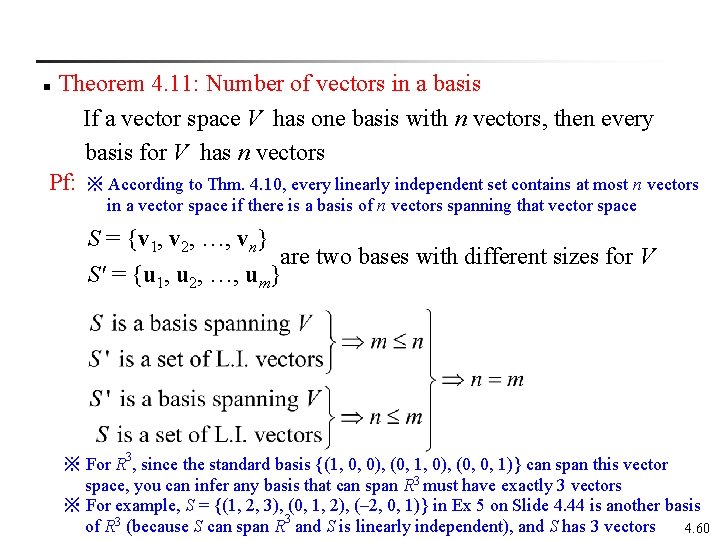
Theorem 4. 11: Number of vectors in a basis If a vector space V has one basis with n vectors, then every basis for V has n vectors Pf: ※ According to Thm. 4. 10, every linearly independent set contains at most n vectors n in a vector space if there is a basis of n vectors spanning that vector space S = {v 1, v 2, …, vn} are two bases with different sizes for V S' = {u 1, u 2, …, um} 3 ※ For R , since the standard basis {(1, 0, 0), (0, 1, 0), (0, 0, 1)} can span this vector space, you can infer any basis that can span R 3 must have exactly 3 vectors ※ For example, S = {(1, 2, 3), (0, 1, 2), (– 2, 0, 1)} in Ex 5 on Slide 4. 44 is another basis of R 3 (because S can span R 3 and S is linearly independent), and S has 3 vectors 4. 60

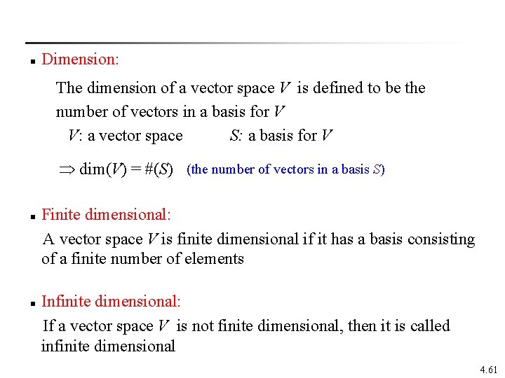
n Dimension: The dimension of a vector space V is defined to be the number of vectors in a basis for V V: a vector space S: a basis for V dim(V) = #(S) (the number of vectors in a basis S) Finite dimensional: A vector space V is finite dimensional if it has a basis consisting of a finite number of elements n Infinite dimensional: If a vector space V is not finite dimensional, then it is called infinite dimensional n 4. 61

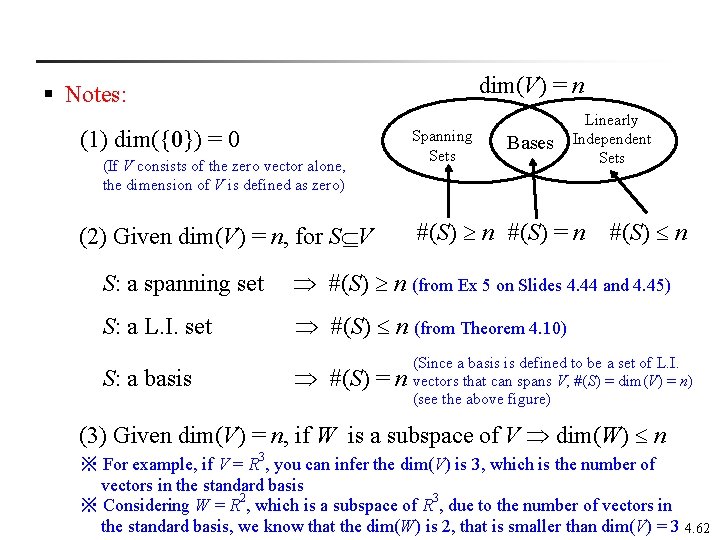
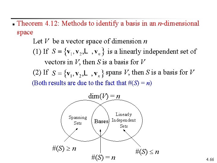
dim(V) = n § Notes: (1) dim({0}) = 0 (If V consists of the zero vector alone, the dimension of V is defined as zero) (2) Given dim(V) = n, for S V Spanning Sets Bases Linearly Independent Sets #(S) n #(S) = n #(S) n S: a spanning set #(S) n (from Ex 5 on Slides 4. 44 and 4. 45) S: a L. I. set #(S) n (from Theorem 4. 10) S: a basis #(S) = n (Since a basis is defined to be a set of L. I. vectors that can spans V, #(S) = dim(V) = n) (see the above figure) (3) Given dim(V) = n, if W is a subspace of V dim(W) n ※ For example, if V = R 3, you can infer the dim(V) is 3, which is the number of vectors in the standard basis ※ Considering W = R 2, which is a subspace of R 3, due to the number of vectors in the standard basis, we know that the dim(W) is 2, that is smaller than dim(V) = 3 4. 62

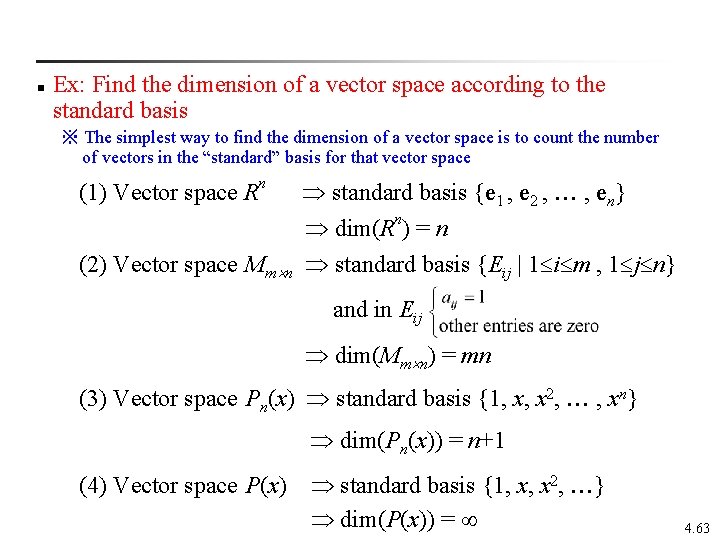
n Ex: Find the dimension of a vector space according to the standard basis ※ The simplest way to find the dimension of a vector space is to count the number of vectors in the “standard” basis for that vector space (1) Vector space Rn standard basis {e 1 , e 2 , , en} dim(Rn) = n (2) Vector space Mm n standard basis {Eij | 1 i m , 1 j n} and in Eij dim(Mm n) = mn (3) Vector space Pn(x) standard basis {1, x, x 2, , xn} dim(Pn(x)) = n+1 (4) Vector space P(x) standard basis {1, x, x 2, } dim(P(x)) = 4. 63

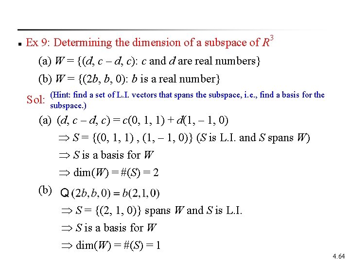
n Ex 9: Determining the dimension of a subspace of R 3 (a) W = {(d, c – d, c): c and d are real numbers} (b) W = {(2 b, b, 0): b is a real number} Sol: (Hint: find a set of L. I. vectors that spans the subspace, i. e. , find a basis for the subspace. ) (a) (d, c – d, c) = c(0, 1, 1) + d(1, – 1, 0) S = {(0, 1, 1) , (1, – 1, 0)} (S is L. I. and S spans W) S is a basis for W dim(W) = #(S) = 2 (b) S = {(2, 1, 0)} spans W and S is L. I. S is a basis for W dim(W) = #(S) = 1 4. 64

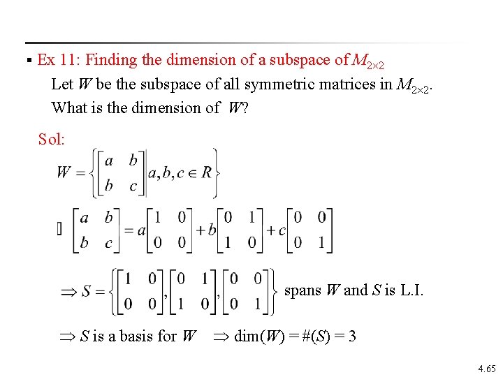
Ex 11: Finding the dimension of a subspace of M 2 2 Let W be the subspace of all symmetric matrices in M 2 2. What is the dimension of W? § Sol: spans W and S is L. I. S is a basis for W dim(W) = #(S) = 3 4. 65

Theorem 4. 12: Methods to identify a basis in an n-dimensional space Let V be a vector space of dimension n (1) If is a linearly independent set of vectors in V, then S is a basis for V (2) If spans V, then S is a basis for V n (Both results are due to the fact that #(S) = n) dim(V) = n Spanning Sets Bases Linearly Independent Sets #(S) n #(S) = n #(S) n 4. 66

6. Rank of a Matrix and Systems of Linear Equations § In this section, three vector spaces are investigated § Row space: the vector space spanned by the row vectors of a matrix A § Column space: the vector space spanned by column vectors of a matrix A § Nullspace: the vector space consisting of all solutions of the homogeneous system of linear equations Ax = 0 § Next, discuss the basis and the dimension of each vector space § Finally, the relationship between the solutions of Ax = b and Ax = 0 will be discussed § To begin the introduction, I present the notation for the row and column vectors of a matrix A with the size m×n on the next slide 4. 67

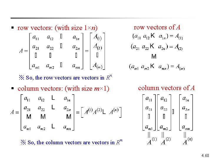
§ row vectors: (with size 1×n) row vectors of A ※ So, the row vectors are vectors in Rn § column vectors: (with size m× 1) ※ So, the column vectors are vectors in Rm column vectors of A || || (1) (2) (n) A A 4. 68

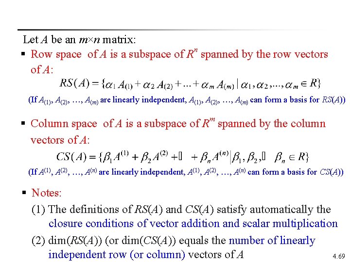
Let A be an m×n matrix: § Row space of A is a subspace of Rn spanned by the row vectors of A: (If A(1), A(2), …, A(m) are linearly independent, A(1), A(2), …, A(m) can form a basis for RS(A)) § Column space of A is a subspace of Rm spanned by the column vectors of A: (If A(1), A(2), …, A(n) are linearly independent, A(1), A(2), …, A(n) can form a basis for CS(A)) § Notes: (1) The definitions of RS(A) and CS(A) satisfy automatically the closure conditions of vector addition and scalar multiplication (2) dim(RS(A)) (or dim(CS(A)) equals the number of linearly independent row (or column) vectors of A 4. 69

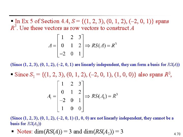
§ In Ex 5 of Section 4. 4, S = {(1, 2, 3), (0, 1, 2), (– 2, 0, 1)} spans R 3. Use these vectors as row vectors to construct A (Since (1, 2, 3), (0, 1, 2), (– 2, 0, 1) are linearly independent, they can form a basis for RS(A)) § Since S 1 = {(1, 2, 3), (0, 1, 2), (– 2, 0, 1), (1, 0, 0)} also spans R 3, (Since (1, 2, 3), (0, 1, 2), (– 2, 0, 1) (1, 0, 0) are not linearly independent, they cannot be a basis for RS(A 1)) § Notes: dim(RS(A)) = 3 and dim(RS(A 1)) = 3 4. 70

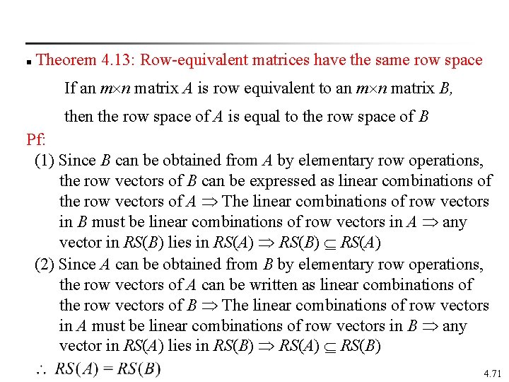
Theorem 4. 13: Row-equivalent matrices have the same row space n If an m n matrix A is row equivalent to an m n matrix B, then the row space of A is equal to the row space of B Pf: (1) Since B can be obtained from A by elementary row operations, the row vectors of B can be expressed as linear combinations of the row vectors of A The linear combinations of row vectors in B must be linear combinations of row vectors in A any vector in RS(B) lies in RS(A) RS(B) RS(A) (2) Since A can be obtained from B by elementary row operations, the row vectors of A can be written as linear combinations of the row vectors of B The linear combinations of row vectors in A must be linear combinations of row vectors in B any vector in RS(A) lies in RS(B) RS(A) RS(B) 4. 71

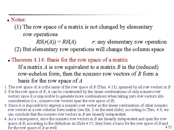
Notes: (1) The row space of a matrix is not changed by elementary row operations RS(r(A)) = RS(A) r: any elementary row operation (2) But elementary row operations will change the column space n n Theorem 4. 14: Basis for the row space of a matrix If a matrix A is row equivalent to a matrix B in the (reduced) row-echelon form, then the nonzero row vectors of B form a basis for the row space of A 1. The row space of A is the same of the row space of B (Thm. 4. 13), spanned by all row vectors in B 2. For the row space of B, it can be constructed by the linear combinations of only nonzero row vectors since it is impossible to generate more combinations when taking zero row vectors into consideration (i. e. , nonzero row vectors span the row space of B) 3. Since it is impossible to express a nonzero row vector as the linear combination of other nonzero row vectors in a row-echelon form matrix (see Ex. 2 on the next slide), according to Thm. 4. 8, we can conclude that the nonzero row vectors in B are linearly independent 4. As a consequence, since the nonzero row vectors in B are linearly independent and span the row space of B, according to the definition on Slide 4. 57, they form a basis for the row space of B and 4. 72 for the row space of A as well

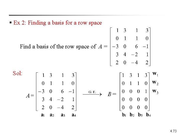
§ Ex 2: Finding a basis for a row space Find a basis of the row space of A = Sol: A= B = 4. 73

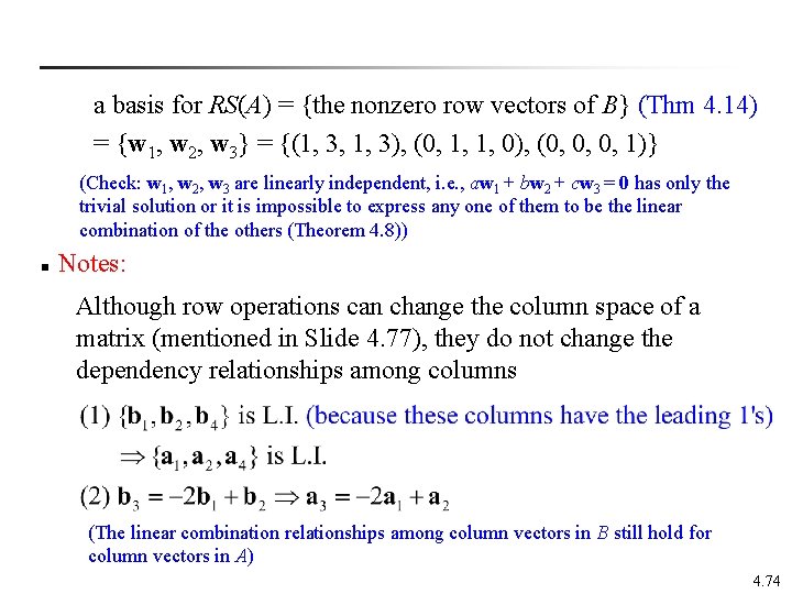
a basis for RS(A) = {the nonzero row vectors of B} (Thm 4. 14) = {w 1, w 2, w 3} = {(1, 3, 1, 3), (0, 1, 1, 0), (0, 0, 0, 1)} (Check: w 1, w 2, w 3 are linearly independent, i. e. , aw 1 + bw 2 + cw 3 = 0 has only the trivial solution or it is impossible to express any one of them to be the linear combination of the others (Theorem 4. 8)) n Notes: Although row operations can change the column space of a matrix (mentioned in Slide 4. 77), they do not change the dependency relationships among columns (The linear combination relationships among column vectors in B still hold for column vectors in A) 4. 74

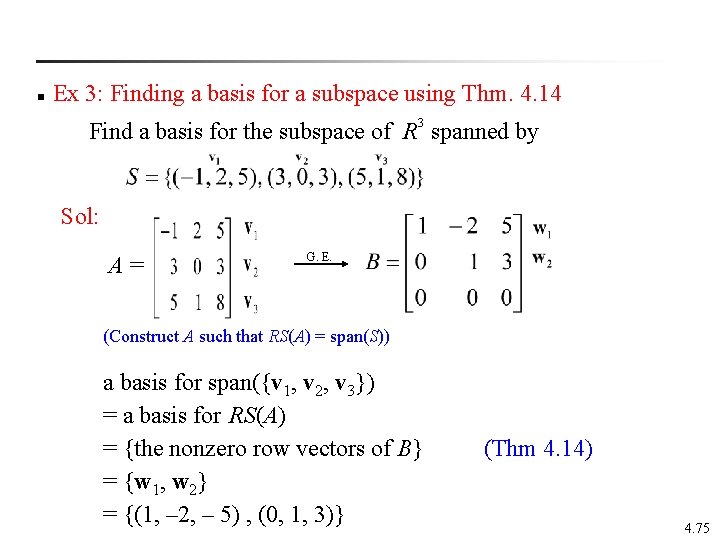
n Ex 3: Finding a basis for a subspace using Thm. 4. 14 Find a basis for the subspace of R 3 spanned by Sol: A= G. E. (Construct A such that RS(A) = span(S)) a basis for span({v 1, v 2, v 3}) = a basis for RS(A) = {the nonzero row vectors of B} (Thm 4. 14) = {w 1, w 2} = {(1, – 2, – 5) , (0, 1, 3)} 4. 75

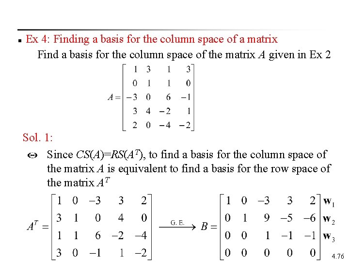
n Ex 4: Finding a basis for the column space of a matrix Find a basis for the column space of the matrix A given in Ex 2 Sol. 1: Since CS(A)=RS(AT), to find a basis for the column space of the matrix A is equivalent to find a basis for the row space of the matrix AT 4. 76

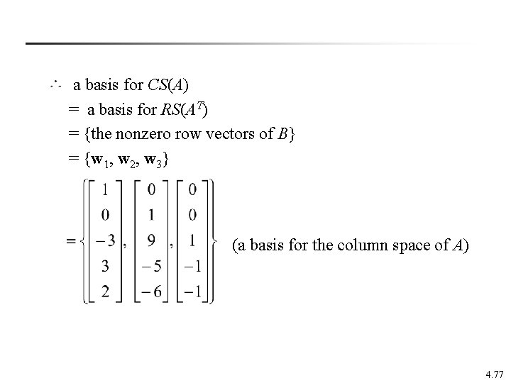
a basis for CS(A) = a basis for RS(AT) = {the nonzero row vectors of B} = {w 1, w 2, w 3} (a basis for the column space of A) 4. 77

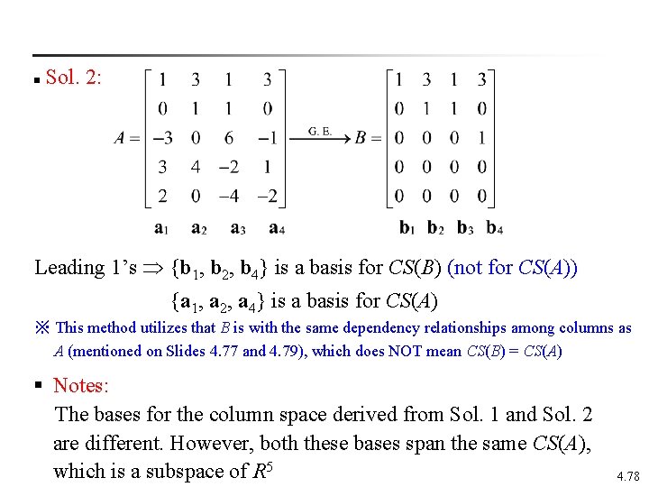
Sol. 2: n Leading 1’s {b 1, b 2, b 4} is a basis for CS(B) (not for CS(A)) {a 1, a 2, a 4} is a basis for CS(A) ※ This method utilizes that B is with the same dependency relationships among columns as A (mentioned on Slides 4. 77 and 4. 79), which does NOT mean CS(B) = CS(A) § Notes: The bases for the column space derived from Sol. 1 and Sol. 2 are different. However, both these bases span the same CS(A), which is a subspace of R 5 4. 78

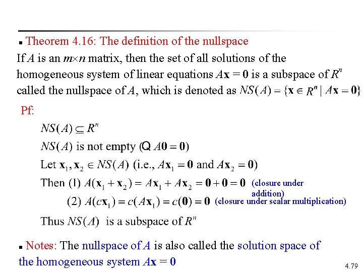
Theorem 4. 16: The definition of the nullspace If A is an m n matrix, then the set of all solutions of the homogeneous system of linear equations Ax = 0 is a subspace of Rn called the nullspace of A, which is denoted as n Pf: (closure under addition) (closure under scalar multiplication) Notes: The nullspace of A is also called the solution space of the homogeneous system Ax = 0 n 4. 79

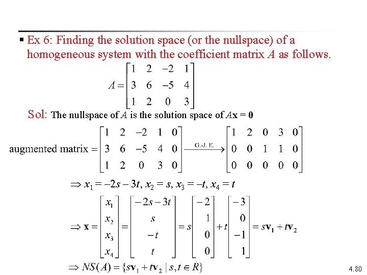
§ Ex 6: Finding the solution space (or the nullspace) of a homogeneous system with the coefficient matrix A as follows. Sol: The nullspace of A is the solution space of Ax = 0 x 1 = – 2 s – 3 t, x 2 = s, x 3 = –t, x 4 = t 4. 80

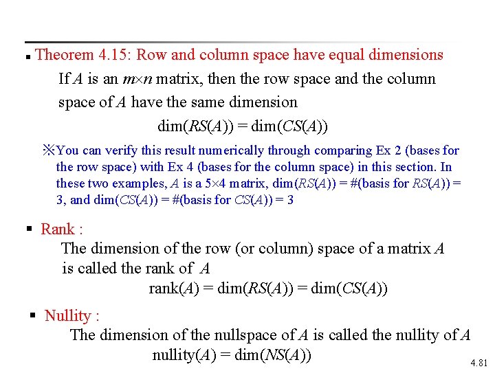
Theorem 4. 15: Row and column space have equal dimensions If A is an m n matrix, then the row space and the column space of A have the same dimension dim(RS(A)) = dim(CS(A)) n ※You can verify this result numerically through comparing Ex 2 (bases for the row space) with Ex 4 (bases for the column space) in this section. In these two examples, A is a 5 4 matrix, dim(RS(A)) = #(basis for RS(A)) = 3, and dim(CS(A)) = #(basis for CS(A)) = 3 § Rank : The dimension of the row (or column) space of a matrix A is called the rank of A rank(A) = dim(RS(A)) = dim(CS(A)) § Nullity : The dimension of the nullspace of A is called the nullity of A nullity(A) = dim(NS(A)) 4. 81

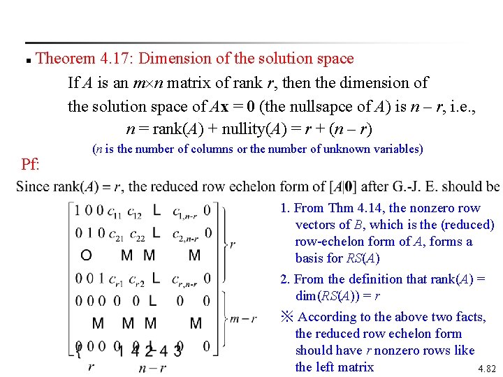
Theorem 4. 17: Dimension of the solution space If A is an m n matrix of rank r, then the dimension of the solution space of Ax = 0 (the nullsapce of A) is n – r, i. e. , n = rank(A) + nullity(A) = r + (n – r) n (n is the number of columns or the number of unknown variables) Pf: 1. From Thm 4. 14, the nonzero row vectors of B, which is the (reduced) row-echelon form of A, forms a basis for RS(A) 2. From the definition that rank(A) = dim(RS(A)) = r ※ According to the above two facts, the reduced row echelon form should have r nonzero rows like the left matrix 4. 82

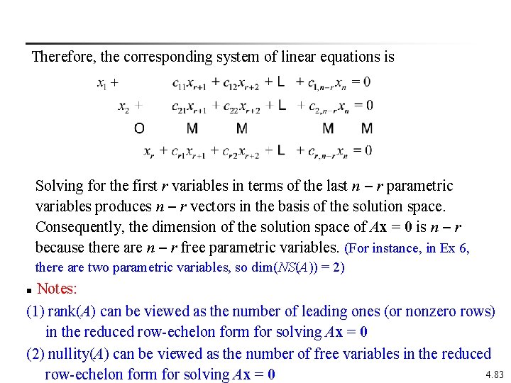
Therefore, the corresponding system of linear equations is Solving for the first r variables in terms of the last n – r parametric variables produces n – r vectors in the basis of the solution space. Consequently, the dimension of the solution space of Ax = 0 is n – r because there are n – r free parametric variables. (For instance, in Ex 6, there are two parametric variables, so dim(NS(A)) = 2) Notes: (1) rank(A) can be viewed as the number of leading ones (or nonzero rows) in the reduced row-echelon form for solving Ax = 0 (2) nullity(A) can be viewed as the number of free variables in the reduced 4. 83 row-echelon form for solving Ax = 0 n

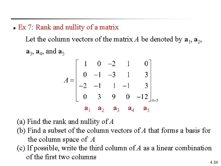
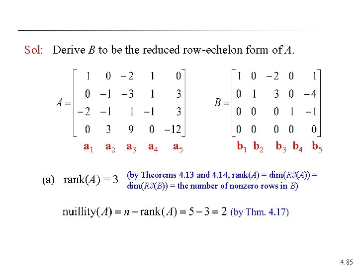
n Ex 7: Rank and nullity of a matrix Let the column vectors of the matrix A be denoted by a 1, a 2, a 3, a 4, and a 5 a 1 a 2 a 3 a 4 a 5 (a) Find the rank and nullity of A (b) Find a subset of the column vectors of A that forms a basis for the column space of A (c) If possible, write third column of A as a linear combination of the first two columns 4. 84

Sol: Derive B to be the reduced row-echelon form of A. a 1 a 2 a 3 a 4 a 5 b 1 b 2 b 3 b 4 b 5 (a) rank(A) = 3 (by Theorems 4. 13 and 4. 14, rank(A) = dim(RS(A)) = dim(RS(B)) = the number of nonzero rows in B) 4. 85

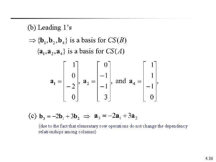
(b) Leading 1’s (c) (due to the fact that elementary row operations do not change the dependency relationships among columns) 4. 86

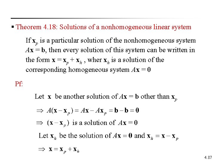
§ Theorem 4. 18: Solutions of a nonhomogeneous linear system If xp is a particular solution of the nonhomogeneous system Ax = b, then every solution of this system can be written in the form x = xp + xh , wher xh is a solution of the corresponding homogeneous system Ax = 0 Pf: Let x be another solution of Ax = b other than xp is a solution of Ax = 0 4. 87

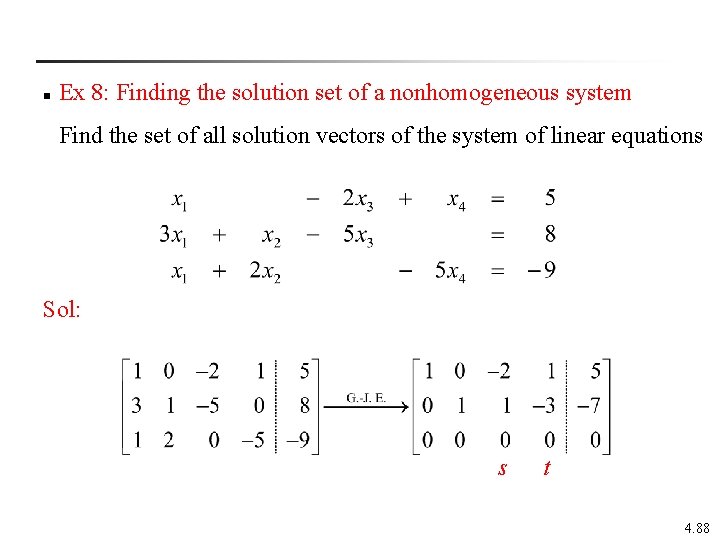
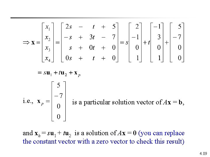
n Ex 8: Finding the solution set of a nonhomogeneous system Find the set of all solution vectors of the system of linear equations Sol: s t 4. 88

i. e. , is a particular solution vector of Ax = b, and xh = su 1 + tu 2 is a solution of Ax = 0 (you can replace the constant vector with a zero vector to check this result) 4. 89

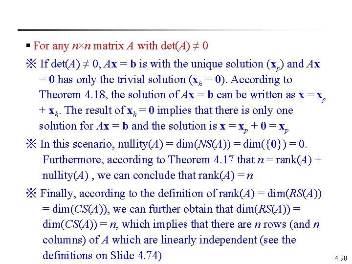
§ For any n×n matrix A with det(A) ≠ 0 ※ If det(A) ≠ 0, Ax = b is with the unique solution (xp) and Ax = 0 has only the trivial solution (xh = 0). According to Theorem 4. 18, the solution of Ax = b can be written as x = xp + xh. The result of xh = 0 implies that there is only one solution for Ax = b and the solution is x = xp + 0 = xp ※ In this scenario, nullity(A) = dim(NS(A)) = dim({0}) = 0. Furthermore, according to Theorem 4. 17 that n = rank(A) + nullity(A) , we can conclude that rank(A) = n ※ Finally, according to the definition of rank(A) = dim(RS(A)) = dim(CS(A)), we can further obtain that dim(RS(A)) = dim(CS(A)) = n, which implies that there are n rows (and n columns) of A which are linearly independent (see the definitions on Slide 4. 74) 4. 90

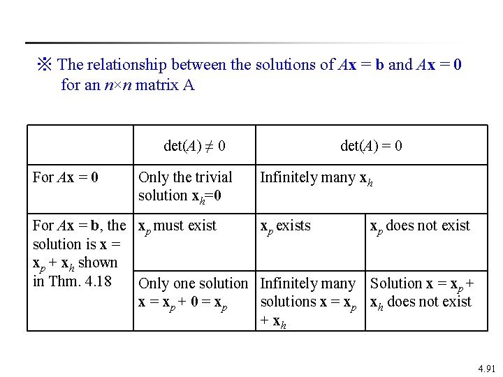
※ The relationship between the solutions of Ax = b and Ax = 0 for an n×n matrix A det(A) ≠ 0 For Ax = 0 Only the trivial solution xh=0 det(A) = 0 Infinitely many xh For Ax = b, the xp must exist xp exists xp does not exist solution is x = xp + xh shown in Thm. 4. 18 Only one solution Infinitely many Solution x = xp + 0 = xp solutions x = xp xh does not exist + xh 4. 91

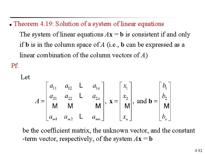
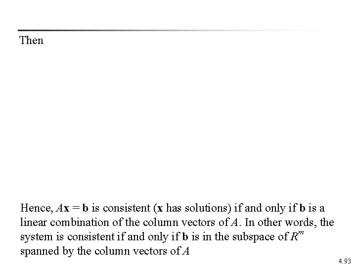
n Theorem 4. 19: Solution of a system of linear equations The system of linear equations Ax = b is consistent if and only if b is in the column space of A (i. e. , b can be expressed as a linear combination of the column vectors of A) Pf: Let be the coefficient matrix, the unknown vector, and the constant -term vector, respectively, of the system Ax = b 4. 92

Then Hence, Ax = b is consistent (x has solutions) if and only if b is a linear combination of the column vectors of A. In other words, the system is consistent if and only if b is in the subspace of Rm spanned by the column vectors of A 4. 93

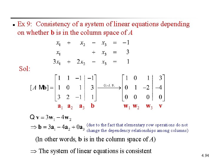
n Ex 9: Consistency of a system of linear equations depending on whether b is in the column space of A Sol: a 1 a 2 a 3 b w 1 w 2 w 3 v (due to the fact that elementary row operations do not change the dependency relationships among columns) (In other words, b is in the column space of A) The system of linear equations is consistent 4. 94

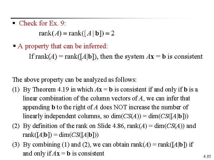
§ Check for Ex. 9: § A property that can be inferred: If rank(A) = rank([A|b]), then the system Ax = b is consistent The above property can be analyzed as follows: (1) By Theorem 4. 19 in which Ax = b is consistent if and only if b is a linear combination of the column vectors of A, we can infer that appending b to the right of A does NOT increase the number of linearly independent columns, so dim(CS(A)) = dim(CS([A|b])) (2) By definition of the rank on Slide 4. 86, rank(A) = dim(CS(A)) and rank([A|b]) = dim(CS([A|b])) (3) By combining (1) and (2), we can obtain rank(A) = rank([A|b]) if and only if Ax = b is consistent 4. 95

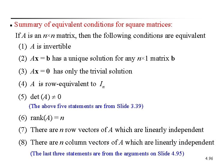
n Summary of equivalent conditions for square matrices: If A is an n×n matrix, then the following conditions are equivalent (1) A is invertible (2) Ax = b has a unique solution for any n× 1 matrix b (3) Ax = 0 has only the trivial solution (4) A is row-equivalent to In (5) det (A) 0 (The above five statements are from Slide 3. 39) (6) rank(A) = n (7) There are n row vectors of A which are linearly independent (8) There are n column vectors of A which are linearly independent (The last three statements are from the arguments on Slide 4. 95) 4. 96

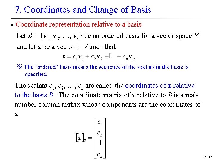
7. Coordinates and Change of Basis n Coordinate representation relative to a basis Let B = {v 1, v 2, …, vn} be an ordered basis for a vector space V and let x be a vector in V such that ※ The “ordered” basis means the sequence of the vectors in the basis is specified The scalars c 1, c 2, …, cn are called the coordinates of x relative to the basis B. The coordinate matrix of x relative to B is a realnumber column matrix whose components are the coordinates of x 4. 97

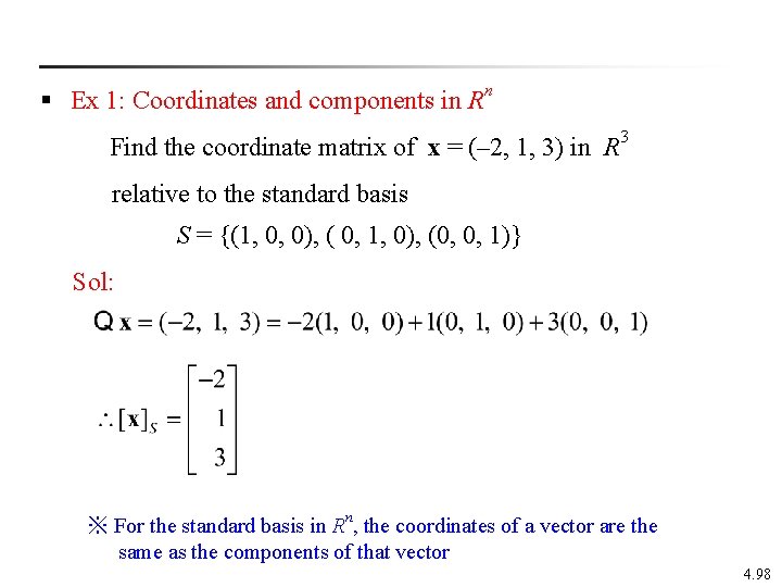
§ Ex 1: Coordinates and components in Rn Find the coordinate matrix of x = (– 2, 1, 3) in R 3 relative to the standard basis S = {(1, 0, 0), ( 0, 1, 0), (0, 0, 1)} Sol: ※ For the standard basis in Rn, the coordinates of a vector are the same as the components of that vector 4. 98

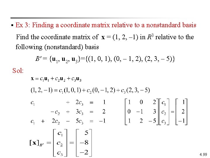
§ Ex 3: Finding a coordinate matrix relative to a nonstandard basis Find the coordinate matrix of x = (1, 2, – 1) in R 3 relative to the following (nonstandard) basis B' = {u 1, u 2, u 3}={(1, 0, 1), (0, – 1, 2), (2, 3, – 5)} Sol: 4. 99

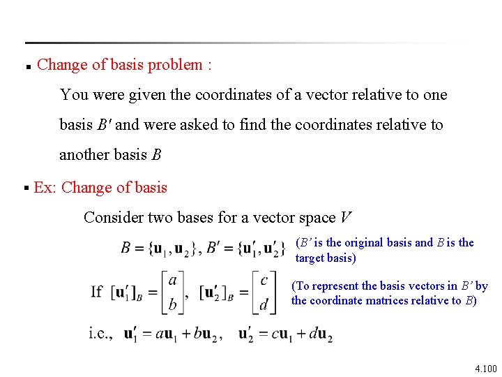
n Change of basis problem : You were given the coordinates of a vector relative to one basis B' and were asked to find the coordinates relative to another basis B § Ex: Change of basis Consider two bases for a vector space V (B’ is the original basis and B is the target basis) (To represent the basis vectors in B’ by the coordinate matrices relative to B) 4. 100

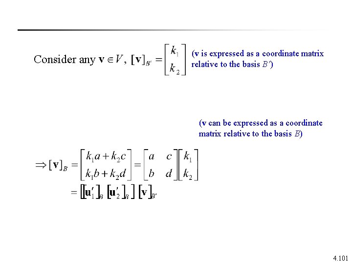
Consider any (v is expressed as a coordinate matrix relative to the basis B’) (v can be expressed as a coordinate matrix relative to the basis B) 4. 101

n Transition matrix from B' to B: If [v]B is the coordinate matrix of v relative to B [v]B’ is the coordinate matrix of v relative to B' (the coordinate matrix relative to the target basis B is derived by multiplying the transition matrix P to the left of the coordinate matrix relative to the original basis B') where is called the transition matrix from B' to B , which is constructed by the coordinate matrices of ordered vectors in B' relative to B 4. 102

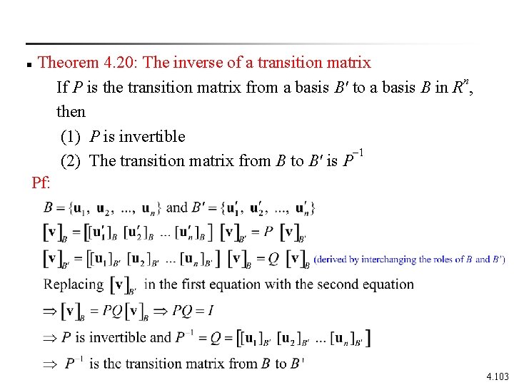
Theorem 4. 20: The inverse of a transition matrix If P is the transition matrix from a basis B' to a basis B in Rn, then (1) P is invertible – 1 (2) The transition matrix from B to B' is P Pf: n 4. 103

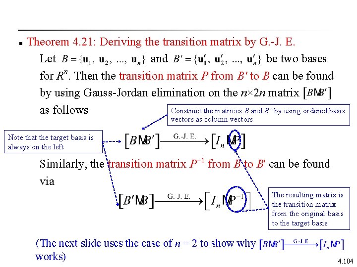
Theorem 4. 21: Deriving the transition matrix by G. -J. E. Let and be two bases for Rn. Then the transition matrix P from B' to B can be found by using Gauss-Jordan elimination on the n× 2 n matrix Construct the matrices B and B’ by using ordered basis as follows n vectors as column vectors Note that the target basis is always on the left Similarly, the transition matrix P– 1 from B to B' can be found via The resulting matrix is the transition matrix from the original basis to the target basis (The next slide uses the case of n = 2 to show why works) 4. 104

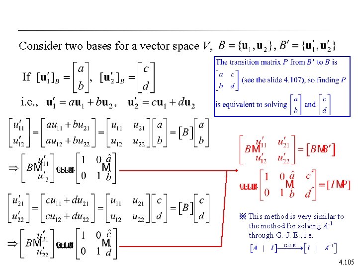
Consider two bases for a vector space V, ※ This method is very similar to the method for solving A-1 through G. -J. E. , i. e. 4. 105

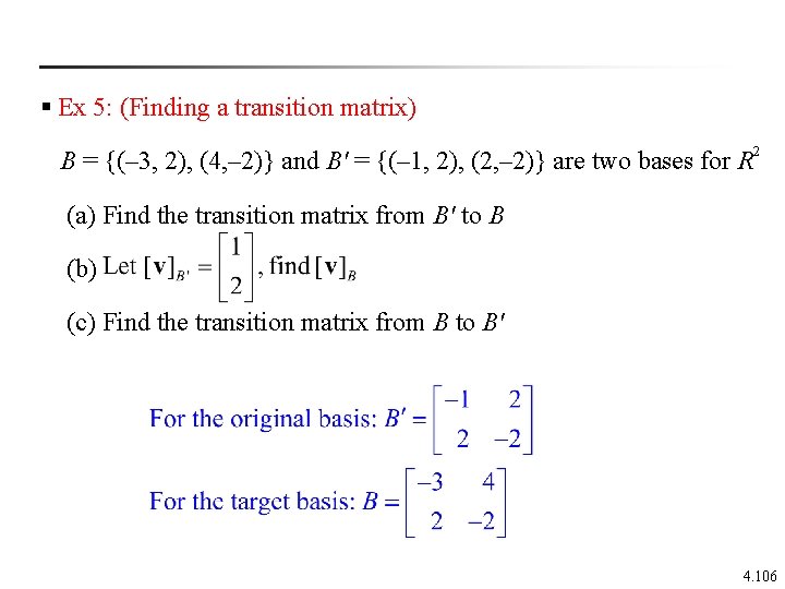
§ Ex 5: (Finding a transition matrix) B = {(– 3, 2), (4, – 2)} and B' = {(– 1, 2), (2, – 2)} are two bases for R 2 (a) Find the transition matrix from B' to B (b) (c) Find the transition matrix from B to B' 4. 106

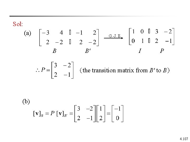
Sol: (a) G. -J. E. B B' I P (the transition matrix from B' to B) (b) 4. 107

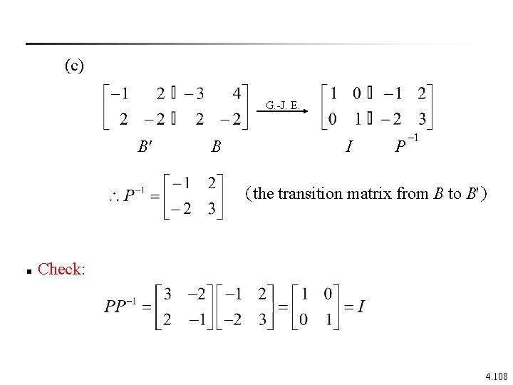
(c) G. -J. E. B' B I P – 1 (the transition matrix from B to B') n Check: 4. 108

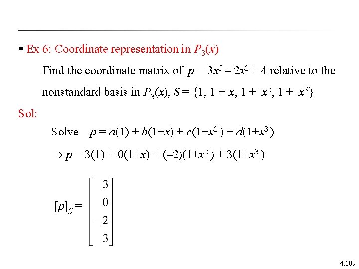
§ Ex 6: Coordinate representation in P 3(x) Find the coordinate matrix of p = 3 x 3 – 2 x 2 + 4 relative to the nonstandard basis in P 3(x), S = {1, 1 + x 2, 1 + x 3} Sol: Solve p = a(1) + b(1+x) + c(1+x 2 ) + d(1+x 3 ) p = 3(1) + 0(1+x) + (– 2)(1+x 2 ) + 3(1+x 3 ) [p]S = 4. 109

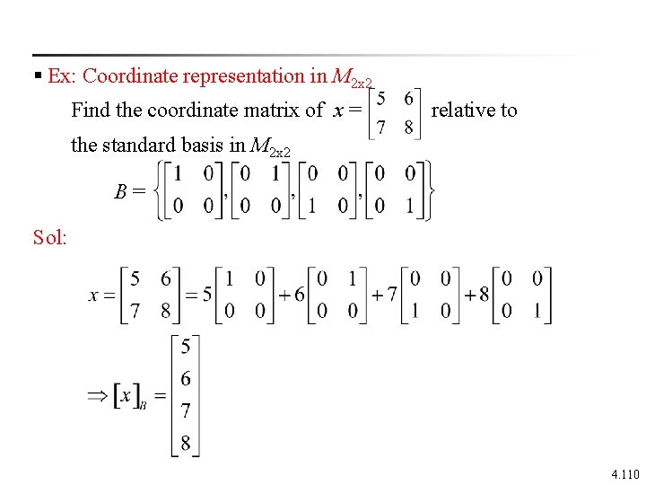
§ Ex: Coordinate representation in M 2 x 2 Find the coordinate matrix of x = relative to the standard basis in M 2 x 2 B = Sol: 4. 110