Random Matrix Theory Random Matrix Theory Shape is

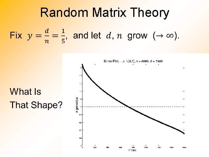
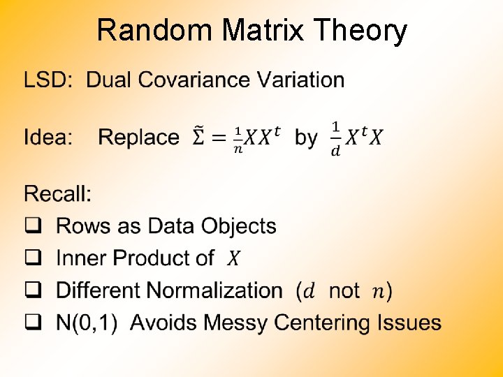
Random Matrix Theory •

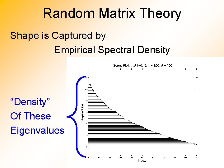
Random Matrix Theory Shape is Captured by Empirical Spectral Density “Density” Of These Eigenvalues

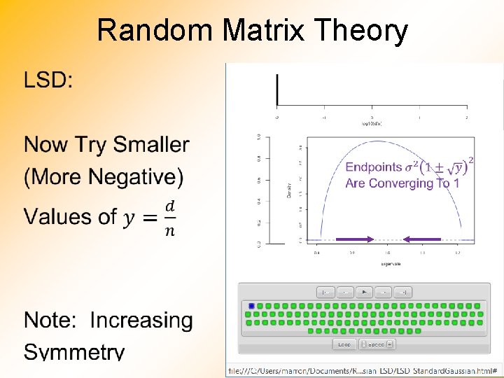
Random Matrix Theory •

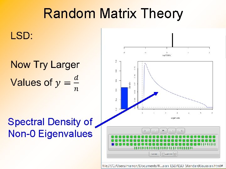
Random Matrix Theory • Spectral Density of Non-0 Eigenvalues

Random Matrix Theory •

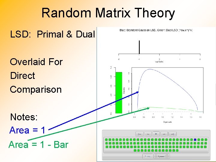
Random Matrix Theory LSD: Primal & Dual Overlaid For Direct Comparison Notes: Area = 1 - Bar

• Discussed on 10/15/19, But Now Know Limit

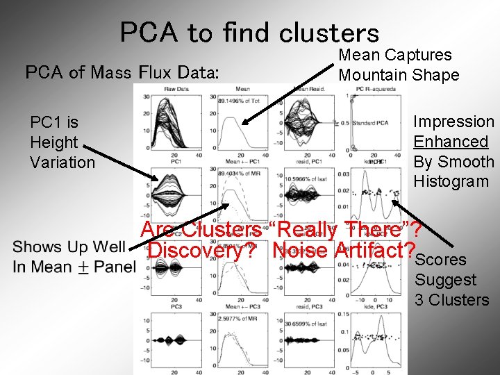
Clusters in data Common Statistical Task: Find Clusters in Data • Interesting sub-populations? • Important structure in data? • How to do this? PCA & visualization is very simple approach There is a large literature of other methods (will study more later)

PCA to find clusters PCA of Mass Flux Data: PC 1 is Height Variation Mean Captures Mountain Shape Impression Enhanced By Smooth Histogram Are Clusters “Really There”? Discovery? Noise Artifact? Scores Suggest 3 Clusters

Statistical Smoothing In 1 Dimension, 2 Major Settings: • Density Estimation “Histograms” • Nonparametric Regression “Scatterplot Smoothing”

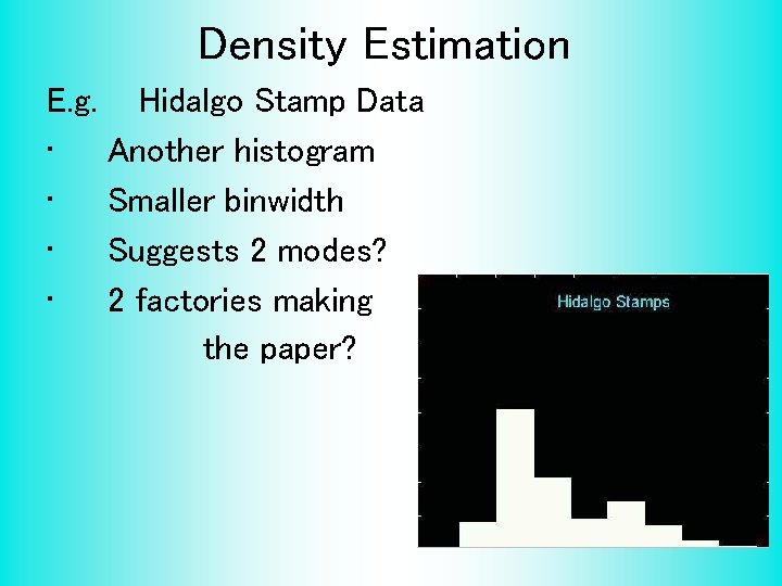
Density Estimation E. g. • • Hidalgo Stamp Data Another histogram Smaller binwidth Suggests 2 modes? 2 factories making the paper?

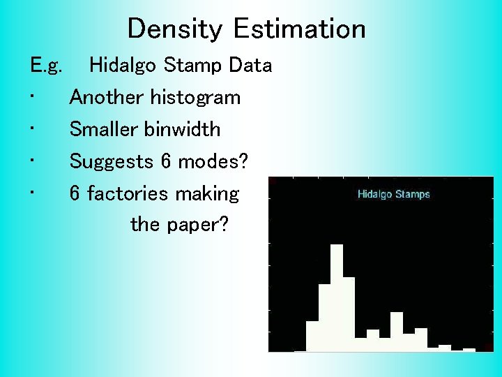
Density Estimation E. g. • • Hidalgo Stamp Data Another histogram Smaller binwidth Suggests 6 modes? 6 factories making the paper?

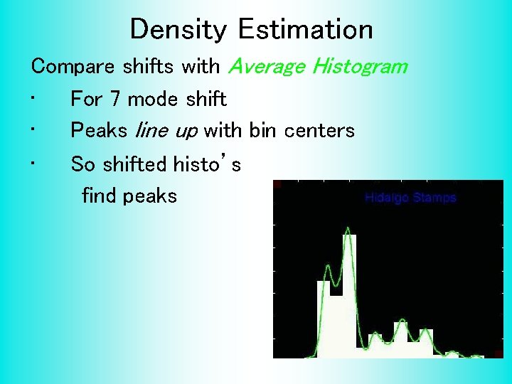
Density Estimation Compare shifts with Average Histogram • For 7 mode shift • Peaks line up with bin centers • So shifted histo’s find peaks

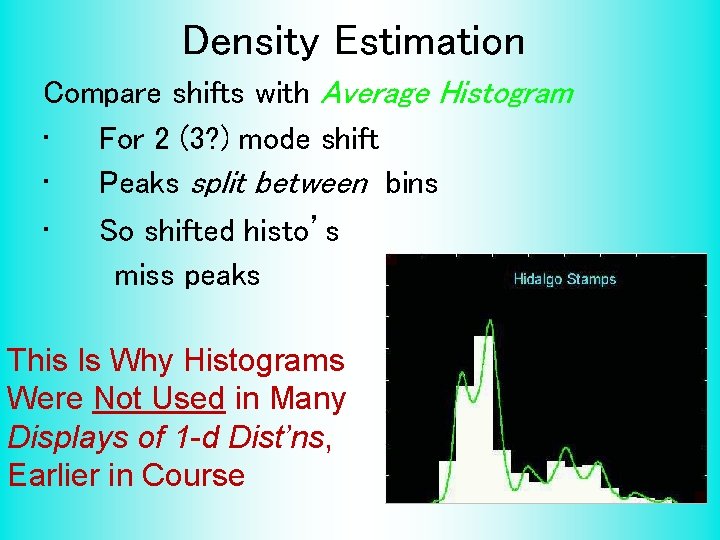
Density Estimation Compare shifts with Average Histogram • For 2 (3? ) mode shift • Peaks split between bins • So shifted histo’s miss peaks This Is Why Histograms Were Not Used in Many Displays of 1 -d Dist’ns, Earlier in Course

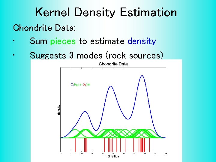
Kernel Density Estimation Chondrite Data: • Sum pieces to estimate density • Suggests 3 modes (rock sources)

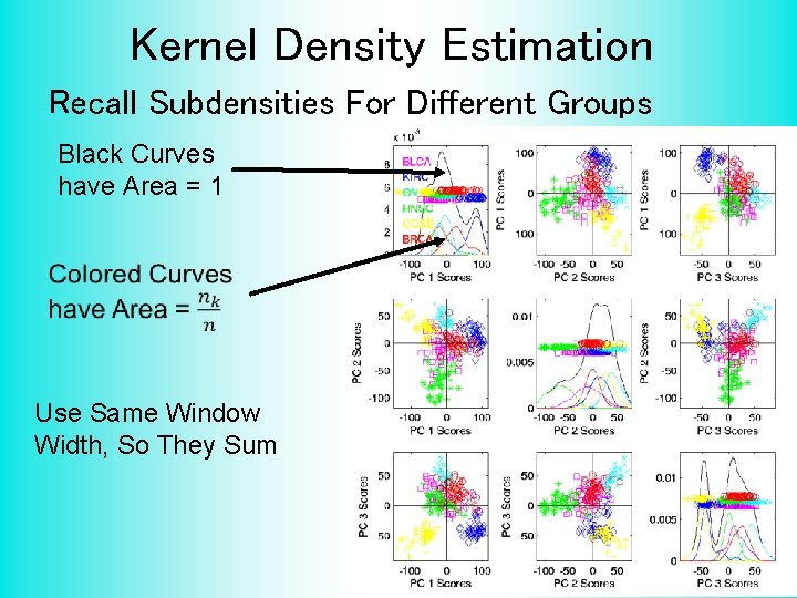
Kernel Density Estimation Recall Subdensities For Different Groups Black Curves have Area = 1 Use Same Window Width, So They Sum

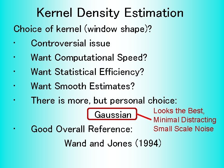
Kernel Density Estimation Choice of kernel (window shape)? • Controversial issue • Want Computational Speed? • Want Statistical Efficiency? • Want Smooth Estimates? • There is more, but personal choice: Looks the Best, Gaussian Minimal Distracting Small Scale Noise • Good Overall Reference: Wand Jones (1994)

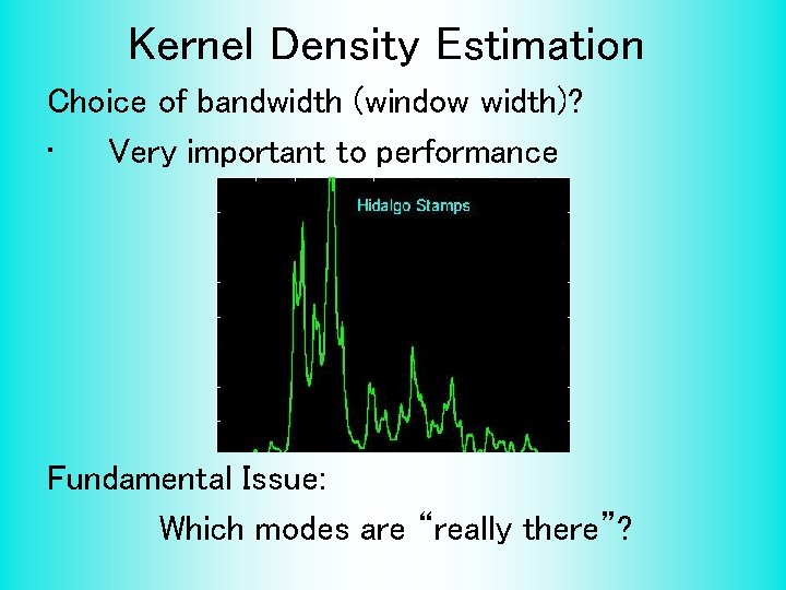
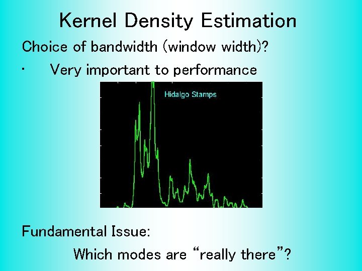
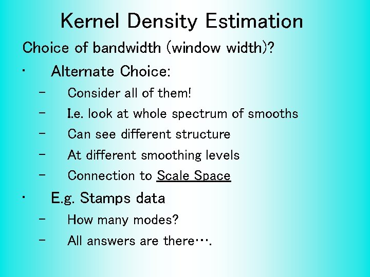
Kernel Density Estimation Choice of bandwidth (window width)? • Very important to performance Fundamental Issue: Which modes are “really there”?

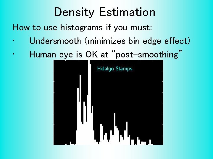
Density Estimation How to use histograms if you must: • Undersmooth (minimizes bin edge effect) • Human eye is OK at “post-smoothing”

Statistical Smoothing 2 Major Settings: • Density Estimation “Histograms” • Nonparametric Regression “Scatterplot Smoothing”

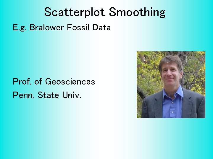
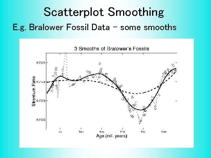
Scatterplot Smoothing E. g. Bralower Fossil Data Prof. of Geosciences Penn. State Univ.

Scatterplot Smoothing E. g. • • • Bralower Fossil Data Study Global Climate Time scale of millions of years Data points are fossil shells Dated by surrounding material Ratio of Isotopes of Strontium Surrogate for Sea Level (Ice Ages)

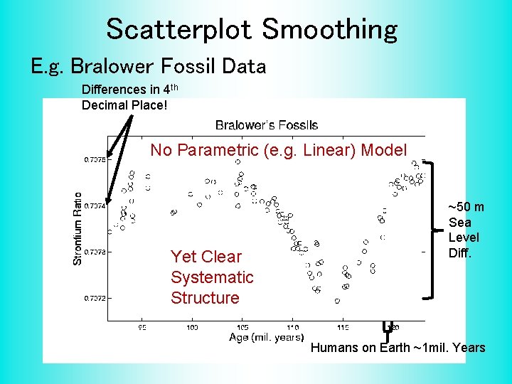
Scatterplot Smoothing E. g. Bralower Fossil Data Differences in 4 th Decimal Place! No Parametric (e. g. Linear) Model Yet Clear Systematic Structure ~50 m Sea Level Diff. Humans on Earth ~1 mil. Years

Scatterplot Smoothing E. g. Bralower Fossil Data • Way to bring out structure: Smooth the data • Methods of smoothing? – – – Local Averages Splines (several types) Fourier – trim high frequencies Other bases … Also controversial

Scatterplot Smoothing E. g. Bralower Fossil Data – some smooths

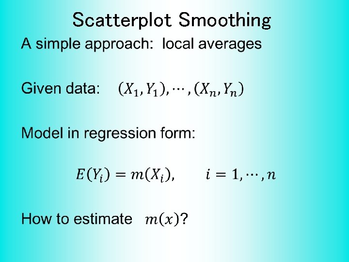
Scatterplot Smoothing •

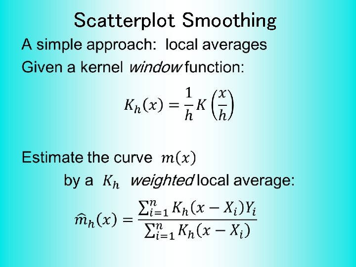
Scatterplot Smoothing •

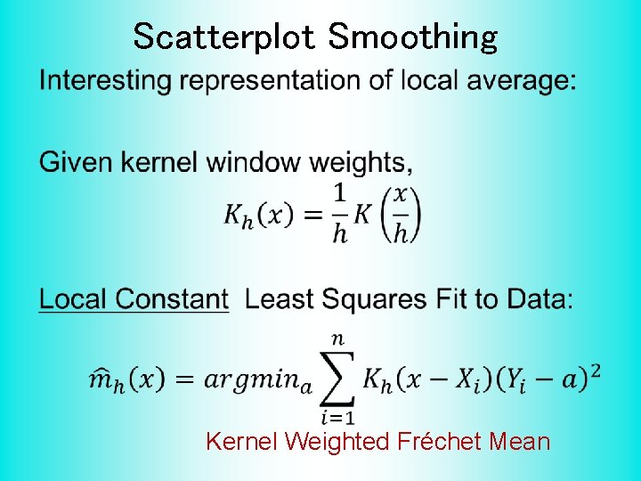
Scatterplot Smoothing • Kernel Weighted Fréchet Mean

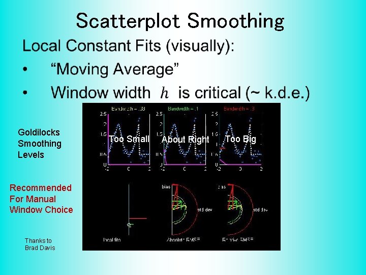
Scatterplot Smoothing • Goldilocks Smoothing Levels Recommended For Manual Window Choice Thanks to Brad Davis Too Small About Right Too Big

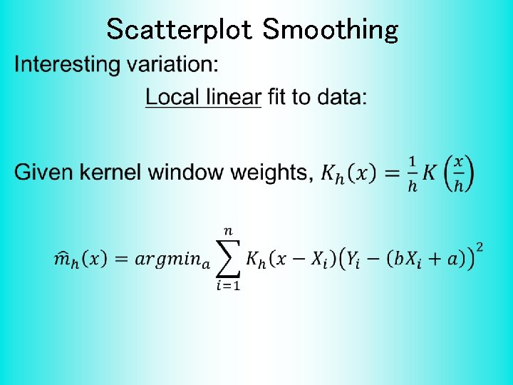
Scatterplot Smoothing •

Scatterplot Smoothing •

Scatterplot Smoothing •

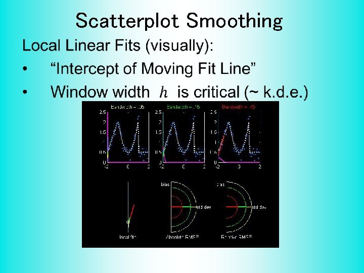
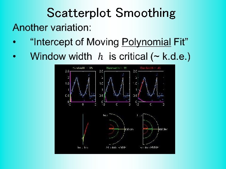
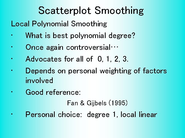
Scatterplot Smoothing Local Polynomial Smoothing • What is best polynomial degree? • Once again controversial… • Advocates for all of 0, 1, 2, 3. • Depends on personal weighting of factors involved • Good reference: Fan & Gijbels (1995) • Personal choice: degree 1, local linear

Scatterplot Smoothing E. g. Bralower Fossils – local linear smooths

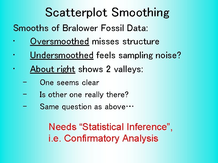
Scatterplot Smoothing Smooths of Bralower Fossil Data: • Oversmoothed misses structure • Undersmoothed feels sampling noise? • About right shows 2 valleys: – – – One seems clear Is other one really there? Same question as above… Needs “Statistical Inference”, i. e. Confirmatory Analysis

Kernel Density Estimation Choice of bandwidth (window width)? • Very important to performance Fundamental Issue: Which modes are “really there”?

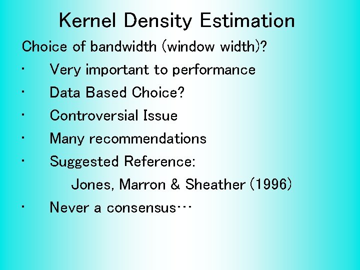
Kernel Density Estimation Choice of bandwidth (window width)? • Very important to performance • Data Based Choice? • Controversial Issue • Many recommendations • Suggested Reference: Jones, Marron & Sheather (1996) • Never a consensus…

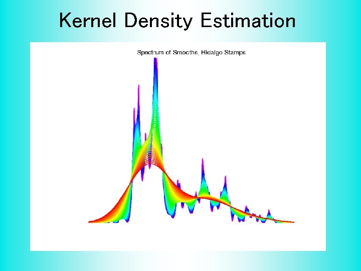
Kernel Density Estimation Choice of bandwidth (window width)? • Alternate Choice: – – – • Consider all of them! I. e. look at whole spectrum of smooths Can see different structure At different smoothing levels Connection to Scale Space E. g. Stamps data – – How many modes? All answers are there….

Kernel Density Estimation

Statistical Smoothing Fundamental Question For both of • Density Estimation: “Histograms” • Regression: “Scatterplot Smoothing” Which bumps are “really there”? vs. “artifacts of sampling noise”?

Si. Zer Background Scale Space – Idea from Computer Vision Goal: Teach Computers to “See” Modern Research: Extract “Information” from Images Early Theoretical work

Si. Zer Background Scale Space – Idea from Computer Vision • Conceptual basis: Oversmoothing = “view from afar” (macroscopic) Undersmoothing = “zoomed in view” (microscopic) Main idea: all smooths contain useful information, so study “full spectrum” (i. e. all smoothing levels) Recommended reference: Lindeberg (1994)

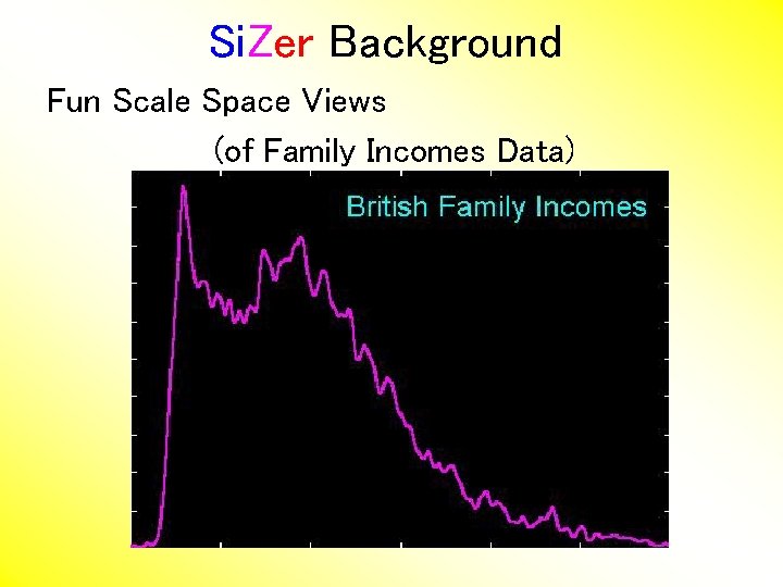
Si. Zer Background Fun Scale Space Views (of Family Incomes Data)

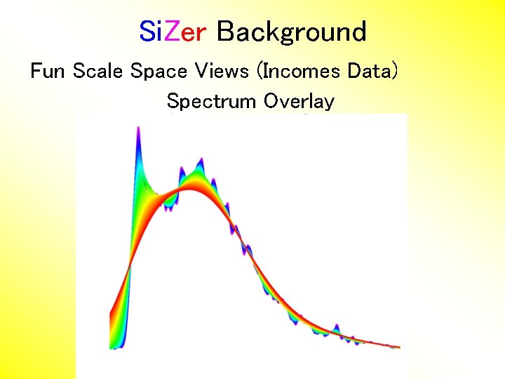
Si. Zer Background Fun Scale Space Views (Incomes Data) Spectrum Overlay

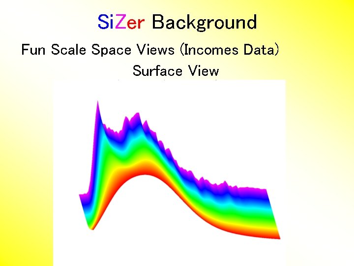
Si. Zer Background Fun Scale Space Views (Incomes Data) Surface View

Si. Zer Background Fun Scale Space Views (of Family Incomes Data) Note: The scale space viewpoint makes Data Dased Bandwidth Selection Much less important (than I once thought…. )

Si. Zer Background Si. Zer: • Significance of Zero crossings, of the derivative, in scale space • Combines: – – • • needed statistical inference novel visualization To get: a powerful exploratory + confirmatory data analysis method Main references: Chaudhuri & Marron (1999) Hannig & Marron (2006)

Si. Zer Background Basic idea: a bump is characterized by: • an increase • followed by a decrease Generalization: Many features of interest captured by sign of the slope of the smooth Foundation of Si. Zer: Statistical inference on slopes, over scale space

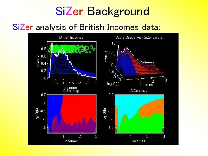
Si. Zer Background Si. Zer Visual presentation: • Color map over scale space: • Blue: slope significantly upwards (derivative CI above 0) • Red: slope significantly downwards (derivative CI below 0) • Purple: slope insignificant (derivative CI contains 0)

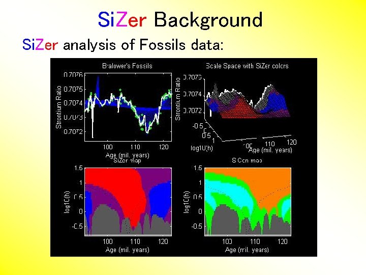
Si. Zer Background Si. Zer analysis of Fossils data:

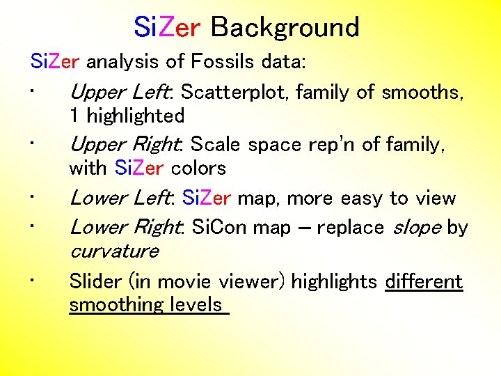
Si. Zer Background Si. Zer analysis of Fossils data: • Upper Left: Scatterplot, family of smooths, 1 highlighted • Upper Right: Scale space rep’n of family, with Si. Zer colors • Lower Left: Si. Zer map, more easy to view • Lower Right: Si. Con map – replace slope by curvature • Slider (in movie viewer) highlights different smoothing levels

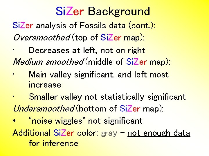
Si. Zer Background Si. Zer analysis of Fossils data (cont. ): Oversmoothed (top of Si. Zer map): • Decreases at left, not on right Medium smoothed (middle of Si. Zer map): • Main valley significant, and left most increase • Smaller valley not statistically significant Undersmoothed (bottom of Si. Zer map): • “noise wiggles” not significant Additional Si. Zer color: gray - not enough data for inference

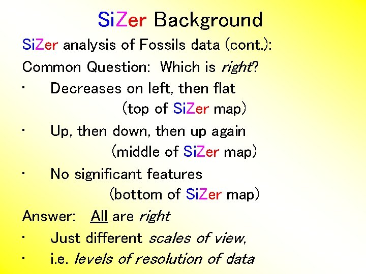
Si. Zer Background Si. Zer analysis of Fossils data (cont. ): Common Question: Which is right? • Decreases on left, then flat (top of Si. Zer map) • Up, then down, then up again (middle of Si. Zer map) • No significant features (bottom of Si. Zer map) Answer: All are right • Just different scales of view, • i. e. levels of resolution of data

Si. Zer Background Si. Zer analysis of British Incomes data:

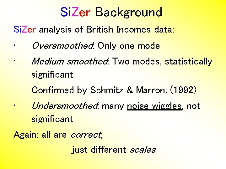
Si. Zer Background Si. Zer analysis of British Incomes data: • • Oversmoothed: Only one mode Medium smoothed: Two modes, statistically significant Confirmed by Schmitz & Marron, (1992) • Undersmoothed: many noise wiggles, not significant Again: all are correct, just different scales

Participant Presentation Wei Gu: A Heuristic Approach to Portfolio Optimization with Cardinality Constraints Nicole Kramer: Calling DNA Loops in Hi-C Data