Propensity Score Matching Summer School for Young Economists

Propensity Score Matching Summer School for Young Economists 2017 June 22, 2017

Today’s Class General Theme: If you don’t have an experiment, how do you get a ‘control group’ p We have already seen D-i-D, RD and others p Another way to get a control group: Matching n Assumptions for identification n Specific form of matching called “propensity score matching” n Is it better than just a plain old regression? p

The Counterfactual Framework p Counterfactual: what would have happened to the treated subjects, had they not received treatment? p Idea: individuals selected into treatment and nontreatment groups have potential outcomes in both states: n n the one in which they are observed the one in which they are not observed.

Reminder of Terms p For the treated group, we have observed mean outcome under the condition of treatment E(Y 1|T=1) and unobserved mean outcome under the condition of nontreatment E(Y 0|T=1). p For the control group we have both observed mean E(Y 0|T=0) and unobserved mean E(Y 1|T=0)

What is “matching”? p Pairing treatment and comparison units that are similar in terms of observable characteristics p Can do this in regressions (with covariates) or prior to regression to define your treatment and control samples

Matching Assumption p Conditioning on observables (X) we can take assignment to treatment ‘as if’ random, i. e. p What is the implicit statement: unobservables (stuff not in X) plays no role in treatment assignment (T)

A matched estimator p E(Y 1 – Y 0 | T=1) = E[Y 1 | X, T=1] – E[Y 0 | X, T=0] E[Y 0 | X, T=1] – E[Y 0 | X, T=0] Assumed to be zero Matched treatment effect Key idea: all selection occurs only through observed X

Common Support p Can only exist if there is a region of “common support” n n p People with the same X values are in both the treatment and the control groups Let S be the set of all observables X, then 0<Pr(T=1 | X)<0 for some S* subset of S Intuition: Someone in control close enough to match to treatment unit OR enough overlap in the distribution of treated and untreated individuals

Lots of common support Between red and blue line is area of common support

Not so much common support

How do we match on p(X) p Taken literally, should match on exactly p(Xi) In practice hard to do so strategy is to match treated units to comparison units whose p-scores are sufficiently close to consider p Issues: p n n n How many times can 1 unit be a “match” How many to match to treatment unit How to “match” if using more than 1 control unit per treatment unit

Replacement p Issue: once control group person Z is a match for individual A, can she also be a match for individual B p Trade-off between bias and precision: n n With replacement minimizes the propensity score distance between the matched and the comparison unit Without replacement

Are we doing a one-to-one match? p If 1 -to-1 match: units closely related but may not be very precise estimates p More you include in match, the more the p -score of the control group will differ from the treatment group p Trade-off between bias and precision n Typically use 1 -to-many match because 1 -to-1 is extremely data intensive if X is multidimensional

Different matching algorithms-1 p Can use nearest neighbor which chooses m closest comparison units n n p Can use ‘caliper’—radius around a point n n p implicitly weights these all the same Get fixed m but may end up with different pscores Again implicitly weights these the same Fixed difference in p-scores, but may not be many units in radius Stratify n n Break sample up into intervals Estimate treatment effect separately in each region

Different Matching Algorithms-2 p Can also use some type of distribution: n Kernel estimator puts some type of distribution (e. g. normal) around the each treatment unit and weights closer control units more and farther control units less n Explicit weighting function can be used if you have some knowledge of how related units of certain distances are to each other

How close is close enough? p No “right” answer in these choices—will depend heavily on sample issues n p How deep is the common support (i. e. are there lots of people in both control and treatment group at all the p-score values Should all be the same asymptotically but in finite samples (which is everything) may differ

Tradeoffs in different methods Source: Caliendo and Kopeinig, 2005

How to estimate a p-score p Typically use a logit n n Specific, useful functional form for estimating “discrete choice” models You haven’t learned these yet but you will p For now, think of running a regular OLS regression where the outcome is 1 if you got the treatment and zero if you didn’t p Take the E[T | X] and that’s your propensity score

The Treatment Effect p p CIA holds and sufficient region of of common support Difference in outcome between treated individual i and weighted comparison group J, with weight generated by the p-score distribution in the common support region N is the treatment group and |N| is the size of the treatment group J is comparison group with |J| is the number of comparison group units matched to i

General Procedure Run Regression: 1 -to-1 match • Dependent variable: T=1, if participate; T = 0, otherwise. Øestimate difference in outcomes for each pair • Choose appropriate conditioning variables, X ØTake average difference as treatment effect • Obtain propensity score: predicted probability (p) 1 -to-n Match Ø Nearest neighbor matching Ø Caliper matching Ø Nonparametric/kernel matching Multivariate analysis based on new sample

Standard Errors p Problem: Estimated variance of treatment effect should include additional variance from estimating p n Typically people “bootstrap” which is a nonparametric form of estimating your coefficients over and over until you get a distribution of those coefficients—use the variance from that

Some concerns about Matching p Data intensive in propensity score estimation n n p May reduce dimensionality of treatment effect estimation but still need enough of a sample to estimate propensity score over common support Need LOTS of X’s for this to be believable Inflexible in how p-score is related to treatment n n Worry about heterogeneity Bias terms much more difficult to sign (nonlinear p-score bias)

Matching + Diff-in-Diff Worry that unobservables causing selection because matching on X not sufficient p Can combine this with difference and difference estimates p n n Take control group J for each individual i Estimate difference before treatment If the groups are truly ‘as if’ random should be zero If it’s not zero: can assume fixed differences over time and take before after difference in treatment and control groups

Calculating Impact using PSM 4. Match Pairs: p Restrict sample to common support (as in Figure) p Need to determine a tolerance limit: how different can control individuals or villages be and still be a match? p Nearest neighbors, nonlinear matching, multiple matches 5. Once matches are made, we can calculate impact by comparing the means of outcomes across participants and their matched pairs

PSM vs Randomization p p Randomization does not require the untestable assumption of independence conditional on observables PSM requires large samples and good data: 1. Ideally, the same data source is used for participants and non-participants 2. Participants and non-participants have access to similar institutions and markets, and 3. The data include X variables capable of identifying program participation and outcomes.

Lessons on Matching Methods p Typically used when neither randomization, RD or other quasi experimental options are not possible n n Case 1: no baseline. Can do ex-post matching Dangers of ex-post matching: Matching on variables that change due to participation (i. e. , endogenous) p What are some variables that won’t change? p p Matching helps control only for OBSERVABLE differences, not unobservable differences

More Lessons on Matching Methods p Matching becomes much better in combination with other techniques, such as: n n p Exploiting baseline data for matching and using difference-in-difference strategy If an assignment rule exists for project, can match on this rule Need good quality data n Common support can be a problem if two groups are very different

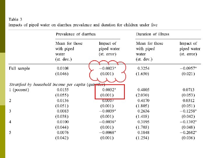
Case Study: Piped Water in India p Jalan and Ravaillion (2003): Impact of piped water for children’s health in rural India p Research questions of interest include: 1. Is a child less vulnerable to diarrhoeal disease if he/she lives in a HH with access to piped water? Do children in poor, or poorly educated, HH have smaller health gains from piped water? Does income matter independently of parental education? 2. 3.

Piped Water: the IE Design p Classic problem for infrastructure programs: randomization is generally not an option (although randomization in timing may be possible in other contexts) p The challenge: observable and unobservable differences across households with piped water and those without n p What are differences for such households in Nigeria? Jalan and Ravallion use cross-sectional data n 1993 -1994 nationally representative survey on 33, 000 rural HH from 1765 villages

PSM in Practice p p To estimate the propensity score, authors used: Village level characteristics Including: Village size, amount of irrigated land, schools, infrastructure (bus stop, railway station) n p Household variables Including: Ethnicity / caste / religion, asset ownership (bicycle, radio, thresher), educational background of HH members n p Are there variables which can not be included? Only using cross-section, so no variables influenced by project n

Piped Water: Behavioral Considerations p IE is designed to estimate not only impact of piped water but to look at how benefits vary across group p There is therefore a behavioral component: poor households may be less able to benefit from piped water b/c they do not properly store water p With this in mind, Are there any key variables missing?

Potential Unobserved Factors p The behavioral factors – importance put on sanitation and behavioral inputs – are also likely correlated with whether a HH has piped water p However, there are no behavioral variables in data: water storage, soap usage, latrines n These are unobserved factors NOT included in propensity score

Piped Water: Impacts p Disease prevalence among those with piped water would be 21% higher without it p Gains from piped water exploited more by wealthier households and households with more educated mothers p Even find counterintuitive result for low income, illiterate HH: piped water is associated with higher diarrhea prevalence

Design When to use Advantages Disadvantages Randomization p. Whenever feasible p. When there is variation at the individual or community level p. Gold standard p. Most powerful p. Not Randomized Encouragement Design p. When an intervention is universally implemented p Provides exogenous variation for a subset of beneficiaries p. Only Regression Discontinuity p. If an intervention has a clear, sharp assignment rule p Project beneficiaries often must qualify through established criteria p. Only Difference-in. Differences p. If two groups are growing at similar rates p Baseline and followup data are available p. Eliminates fixed differences not related to treatment p. Can Matching p When other methods are not possible p. Overcomes p. Assumes observed differences between treatment and comparison always feasible p. Not always ethical looks at subgroup of sample p. Power of encouragement design only known ex post look at subgroup of sample p. Assignment rule in practice often not implemented strictly be biased if trends change p. Ideally have 2 preintervention periods of data no unobserved differences (often implausible)