The central role of the propensity score in

The central role of the propensity score in observational studies for causal effects Rosenbaum PR, Rubin DB (1983). Biometrika 70: 41 -55.

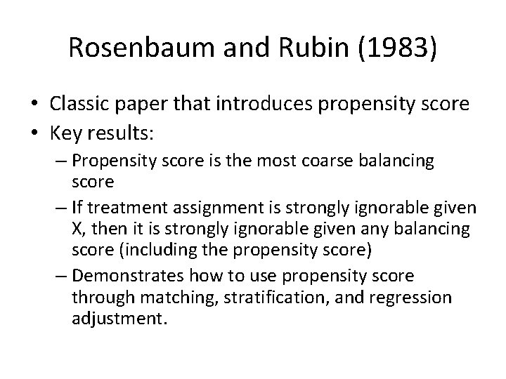
Rosenbaum and Rubin (1983) • Classic paper that introduces propensity score • Key results: – Propensity score is the most coarse balancing score – If treatment assignment is strongly ignorable given X, then it is strongly ignorable given any balancing score (including the propensity score) – Demonstrates how to use propensity score through matching, stratification, and regression adjustment.

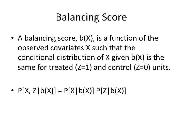
Balancing Score • A balancing score, b(X), is a function of the observed covariates X such that the conditional distribution of X given b(X) is the same for treated (Z=1) and control (Z=0) units. • P[X, Z|b(X)] = P[X|b(X)] P[Z|b(X)]

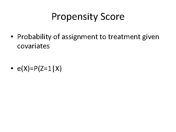
Propensity Score • Probability of assignment to treatment given covariates • e(X)=P(Z=1|X)

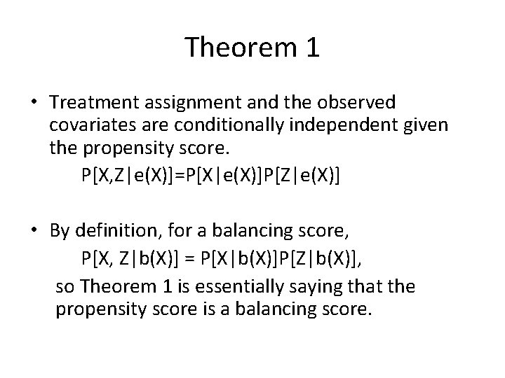
Theorem 1 • Treatment assignment and the observed covariates are conditionally independent given the propensity score. P[X, Z|e(X)]=P[X|e(X)]P[Z|e(X)] • By definition, for a balancing score, P[X, Z|b(X)] = P[X|b(X)]P[Z|b(X)], so Theorem 1 is essentially saying that the propensity score is a balancing score.

Proof that the propensity score is a balancing score • Show that P[X, Z|e(X)]=P[X|e(X)]P[Z|e(X)] or equivalently, P[Z=1|X, e(X)]=P[Z=1|e(X)]. • P[Z=1|X, e(X)]=P[Z=1|X]=e(X), and • P[Z=1|e(X)]=E[Z|e(X)] =E{E[Z|X, e(X)]|X} =E{E[Z|X]|X} =E{e(X)|X} =e(X). • Therefore, P[Z=1|X, e(X)]=P[Z=1|e(X)], and e(X) is a balancing score.

Theorem 2 • b(X) is a balancing score, that is, P[X, Z|b(X)]=P[X|b(X)]P[Z|b(X)], if and only if b(X) is finer than e(X) in the sense that e(X)=f[b(X)] for some function f. • This theorem states that the propensity score is the most coarse balancing score.

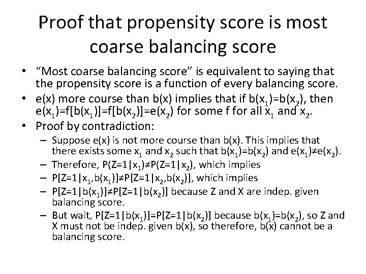
Proof that propensity score is most coarse balancing score • “Most coarse balancing score” is equivalent to saying that the propensity score is a function of every balancing score. • e(x) more course than b(x) implies that if b(x 1)=b(x 2), then e(x 1)=f[b(x 1)]=f[b(x 2)]=e(x 2) for some f for all x 1 and x 2. • Proof by contradiction: – Suppose e(x) is not more course than b(x). This implies that there exists some x 1 and x 2 such that b(x 1)=b(x 2) and e(x 1)≠e(x 2). – Therefore, P(Z=1|x 1)≠P(Z=1|x 2), which implies – P[Z=1|x 1, b(x 1)]≠P[Z=1|x 2, b(x 2)], which implies – P[Z=1|b(x 1)]≠P[Z=1|b(x 2)] because Z and X are indep. given balancing score. – But wait, P[Z=1|b(x 1)]=P[Z=1|b(x 2)] because b(x 1)=b(x 2), so Z and X must not be indep. given b(x), so therefore, b(x) cannot be a balancing score.

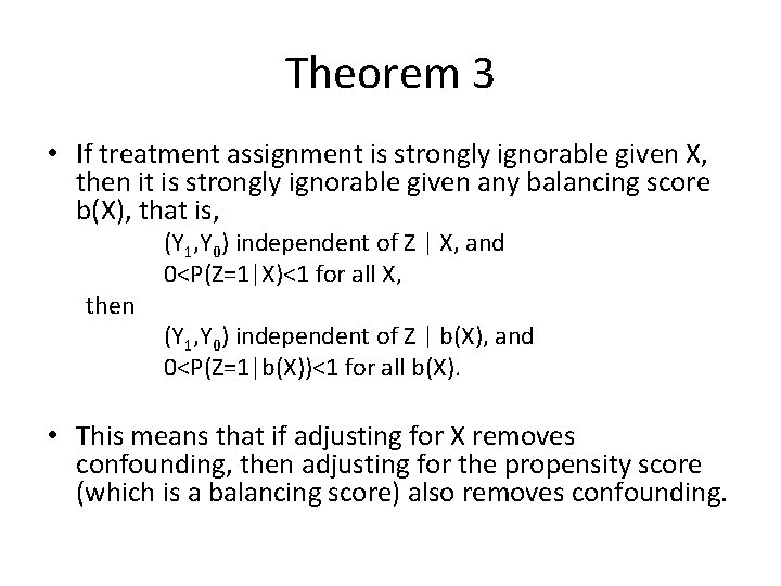
Theorem 3 • If treatment assignment is strongly ignorable given X, then it is strongly ignorable given any balancing score b(X), that is, then (Y 1, Y 0) independent of Z | X, and 0<P(Z=1|X)<1 for all X, (Y 1, Y 0) independent of Z | b(X), and 0<P(Z=1|b(X))<1 for all b(X). • This means that if adjusting for X removes confounding, then adjusting for the propensity score (which is a balancing score) also removes confounding.

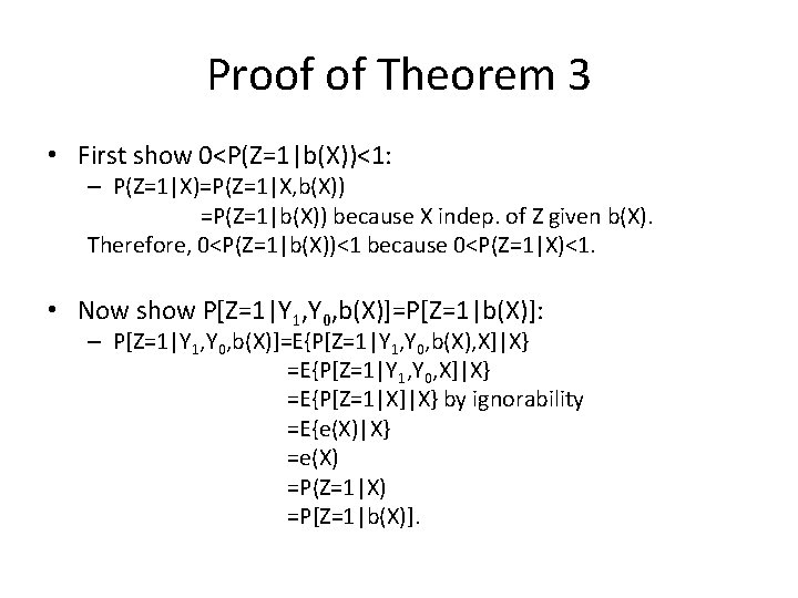
Proof of Theorem 3 • First show 0<P(Z=1|b(X))<1: – P(Z=1|X)=P(Z=1|X, b(X)) =P(Z=1|b(X)) because X indep. of Z given b(X). Therefore, 0<P(Z=1|b(X))<1 because 0<P(Z=1|X)<1. • Now show P[Z=1|Y 1, Y 0, b(X)]=P[Z=1|b(X)]: – P[Z=1|Y 1, Y 0, b(X)]=E{P[Z=1|Y 1, Y 0, b(X), X]|X} =E{P[Z=1|Y 1, Y 0, X]|X} =E{P[Z=1|X]|X} by ignorability =E{e(X)|X} =e(X) =P(Z=1|X) =P[Z=1|b(X)].

Average Treatment Effect (Theorem 4) • E[Y 1 -Y 0] is what we want. • E[Y 1|Z=1]-E[Y 0|Z=0] is what we observe. • If treatment assignment is strongly ignorable given X, then E {E[Y 1|X, Z=1]-E[Y 0|X, Z=0]} =E{E[Y 1|X]-E[Y 0|X]} =E[Y 1 -Y 0]. • Similarly, E {E[Y 1|b(X), Z=1]-E[Y 0|b(X), Z=0]} =E{E[Y 1|b(X)]-E[Y 0|b(X)]} =E[Y 1 -Y 0].

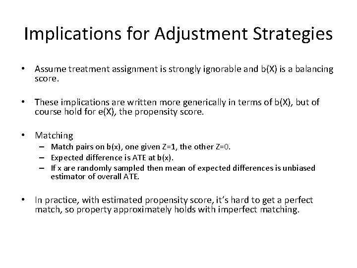
Implications for Adjustment Strategies • Assume treatment assignment is strongly ignorable and b(X) is a balancing score. • These implications are written more generically in terms of b(X), but of course hold for e(X), the propensity score. • Matching – Match pairs on b(x), one given Z=1, the other Z=0. – Expected difference is ATE at b(x). – If x are randomly sampled then mean of expected differences is unbiased estimator of overall ATE. • In practice, with estimated propensity score, it’s hard to get a perfect match, so property approximately holds with imperfect matching.

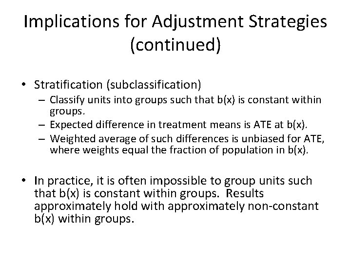
Implications for Adjustment Strategies (continued) • Stratification (subclassification) – Classify units into groups such that b(x) is constant within groups. – Expected difference in treatment means is ATE at b(x). – Weighted average of such differences is unbiased for ATE, where weights equal the fraction of population in b(x). • In practice, it is often impossible to group units such that b(x) is constant within groups. Results approximately hold with approximately non-constant b(x) within groups.

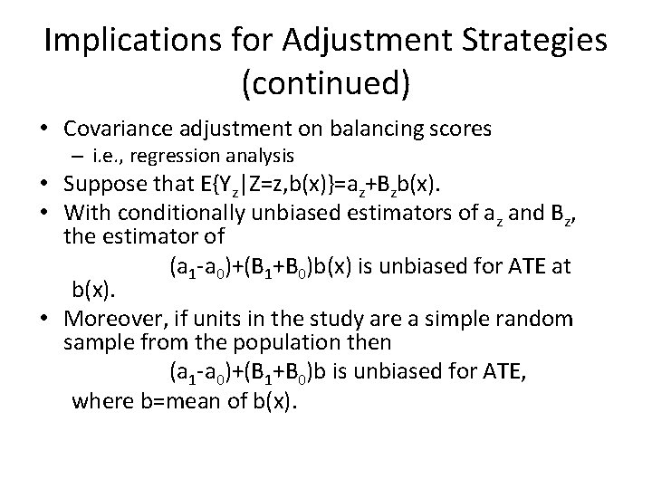
Implications for Adjustment Strategies (continued) • Covariance adjustment on balancing scores – i. e. , regression analysis • Suppose that E{Yz|Z=z, b(x)}=az+Bzb(x). • With conditionally unbiased estimators of az and Bz, the estimator of (a 1 -a 0)+(B 1+B 0)b(x) is unbiased for ATE at b(x). • Moreover, if units in the study are a simple random sample from the population then (a 1 -a 0)+(B 1+B 0)b is unbiased for ATE, where b=mean of b(x).

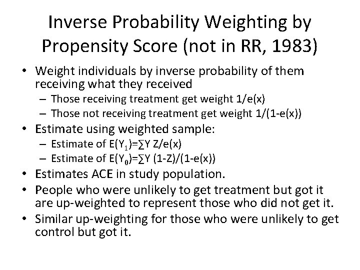
Inverse Probability Weighting by Propensity Score (not in RR, 1983) • Weight individuals by inverse probability of them receiving what they received – Those receiving treatment get weight 1/e(x) – Those not receiving treatment get weight 1/(1 -e(x)) • Estimate using weighted sample: – Estimate of E(Y 1)=∑Y Z/e(x) – Estimate of E(Y 0)=∑Y (1 -Z)/(1 -e(x)) • Estimates ACE in study population. • People who were unlikely to get treatment but got it are up-weighted to represent those who did not get it. • Similar up-weighting for those who were unlikely to get control but got it.

Proof that IPW estimate is unbiased estimate of causal effect • E[Y Z /e(X)] = E{E[Y Z /e(X) |X]} = E{E[Y 1|X] E[Z|X] /e(X)]} = E{E[Y 1|X]} = E[Y 1] Line 2 is by consistency, line 3 is by conditional ignorability, line 4 is by definition of propensity score; Proof similar for E{Y(1 -Z)/[1 -e(x)]}=E[Y 0].

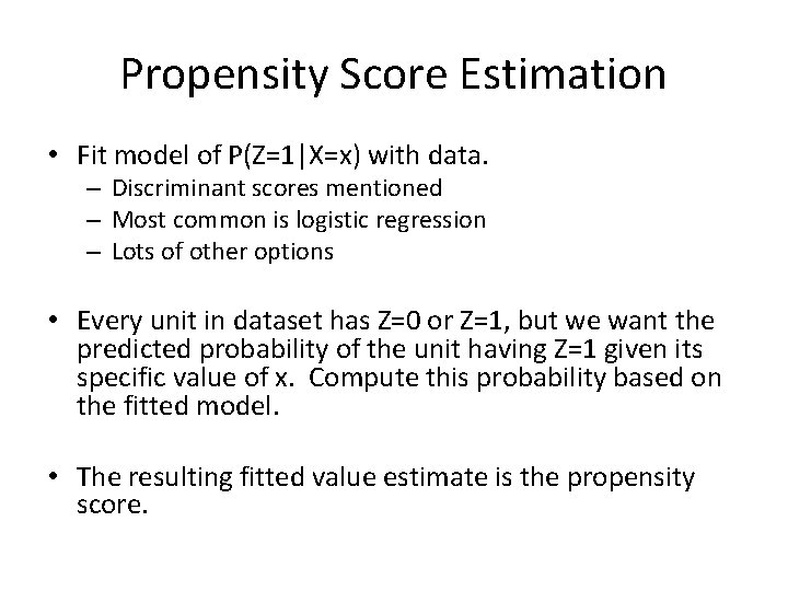
Propensity Score Estimation • Fit model of P(Z=1|X=x) with data. – Discriminant scores mentioned – Most common is logistic regression – Lots of other options • Every unit in dataset has Z=0 or Z=1, but we want the predicted probability of the unit having Z=1 given its specific value of x. Compute this probability based on the fitted model. • The resulting fitted value estimate is the propensity score.

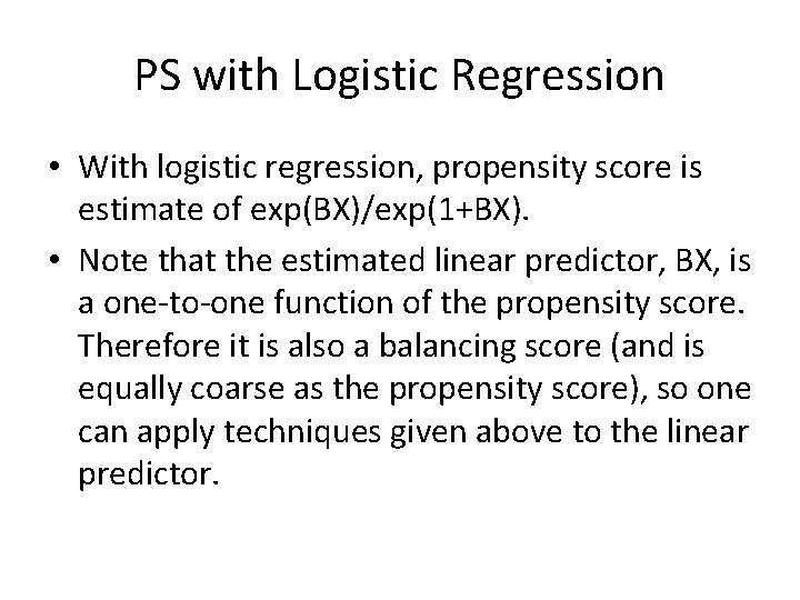
PS with Logistic Regression • With logistic regression, propensity score is estimate of exp(BX)/exp(1+BX). • Note that the estimated linear predictor, BX, is a one-to-one function of the propensity score. Therefore it is also a balancing score (and is equally coarse as the propensity score), so one can apply techniques given above to the linear predictor.