Applying Propensity Score Matching Methods in Institutional Research

Applying Propensity Score Matching Methods in Institutional Research Stephen L. Des. Jardins Professor Center for the Study of Higher and Postsecondary Education School of Education and Professor, Gerald R. Ford School of Public Policy University of Michigan CA AIR Conference Workshop November 20, 2014 1

Organization of the Workshop • Examine conceptual basis of nonexperimental methods – This is a necessary but not sufficient condition for conducting methodologically rigorous research • Survey conceptual foundations of matching methods, esp. PSM methods • Provide & discuss Stata commands to estimate PSM models • Share references to readings & sources of code to enhance post-workshop learning 2

Importance of Rigor in Research • Systematically improving education policies, programs, practices requires understanding of “what works” • Goal: Make causal statements – Without doing so “it is difficult to accumulate a knowledge base that has value for practice or future study” (Schneider, 2007, p. 2). • However, education research has lacked rigor & relevance Quote 3

Why the Lack of Rigor? • Often lack of clarity about the designs & methods optimal for making causal claims • Many researchers were not educated in the application of these methods • Many lack time to learn new methods; may feel they are to complicated to learn • Hard to create & sustain norms & common discourse about what constitutes rigor 4

Policy Changes Driving Push Toward Rigor • NCLB Act (2001): Included definition of “scientifically-based” research & set aside funds for studies consistent with definition • Education Sciences Reform Act (2002) replaced Office of Ed Research & Improvement (OERI) with IES • Funding from IES, NSF, & other federal agencies tied to rigorous designs/methods • Many reports focused on need to improve the quality of education research 5

Cause and Effect • In randomized control trials (RCTs) the question is: What is effect of a specific program or intervention? • Summer Bridge program (intervention) may cause an effect (improved college readiness) • Shadish, Cook, & Campbell (2002): Rarely know all the causes of effects or how they relate to one another – Need for controls in regression frameworks 6

Cause and Effect (cont’d) • Holland (1986) notes that true causes hard to determine unequivocally; seek to determine probability that an effect will occur • Allows opportunity to est. why some effects occur in some situations but not in others – Example: Completing higher levels of math courses in HS may improve chances of finishing college more for some students than for others – Here we are measuring likelihood that cause led to the effect; not “true” cause/effect 7

Determining Causation • RCTs are the “gold standard” to determine causal effects • Pros: Reduce bias & spurious findings, thereby improving knowledge of what works • Cons: Ethics, external validity, cost, errors that are also inherent in observational studies – Measurement problems; “spillover” effects, attrition • Possibilities: Oversubscribed programs (Living Learning Communities, UROP…) 8

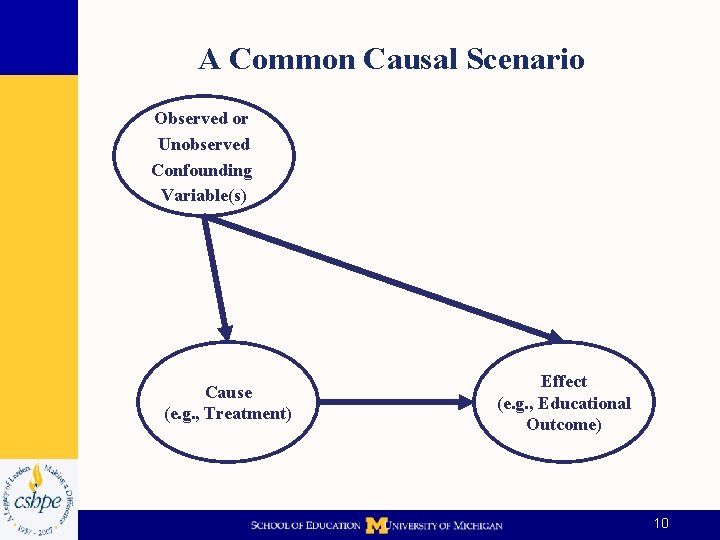
The Logic of Causal Inference • Need to distinguish between inference model specifying cause/effect relation & statistical methods determining strength of relation • The inference model specifies the parameters we want to estimate or test • The statistical technique describes the mathematical procedure(s) to test hypotheses about whether a treatment produces an effect 9

A Common Causal Scenario Observed or Unobserved Confounding Variable(s) Cause (e. g. , Treatment) Effect (e. g. , Educational Outcome) 10

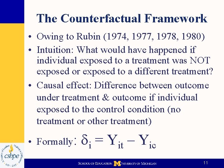
The Counterfactual Framework • Owing to Rubin (1974, 1977, 1978, 1980) • Intuition: What would have happened if individual exposed to a treatment was NOT exposed or exposed to a different treatment? • Causal effect: Difference between outcome under treatment & outcome if individual exposed to the control condition (no treatment or other treatment) • Formally: di = Yit – Yic 11

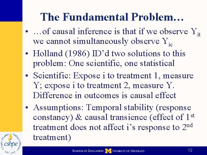
The Fundamental Problem… • …of causal inference is that if we observe Yit we cannot simultaneously observe Yic • Holland (1986) ID’d two solutions to this problem: One scientific, one statistical • Scientific: Expose i to treatment 1, measure Y; expose i to treatment 2, measure Y. Difference in outcomes is causal effect • Assumptions: Temporal stability (response constancy) & causal transience (effect of 1 st treatment does not affect i’s response to 2 nd treatment) 12

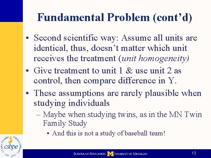
Fundamental Problem (cont’d) • Second scientific way: Assume all units are identical, thus, doesn’t matter which unit receives the treatment (unit homogeneity) • Give treatment to unit 1 & use unit 2 as control, then compare difference in Y. • These assumptions are rarely plausible when studying individuals – Maybe when studying twins, as in the MN Twin Family Study • And this is not a study of baseball team! 13

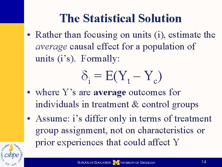
The Statistical Solution • Rather than focusing on units (i), estimate the average causal effect for a population of units (i’s). Formally: di = E(Yt – Yc) • where Y’s are average outcomes for individuals in treatment & control groups • Assume: i’s differ only in terms of treatment group assignment, not on characteristics or prior experiences that could affect Y 14

Example • If we study the effects of being in a summer bridge program on GPA in 1 st semester of college, maybe students who select into treatment are materially different than peers • If we could randomly assign students to the program (or not) then we could examine causal impact of program on GPA. • Why? Because group assignment would, on average, be independent of any measured or unmeasured pretreatment characteristics. 15

Problems with Idealized Solution • Random assignment not always possible, so pretreatment characteristics & treatment group assignment independence violated • Even when randomization is used, statistical methods are often used to adjust for confounding variables – By controlling for student, classroom, school characteristics that predict treatment assignment & outcomes – But this approach is often sub-optimal 16

Criteria for Making Causal Statements • Causal relativity: Effect of cause must be made compared to effect of another cause • Causal manipulation: Units must be potentially exposable to both the treatment & control conditions. • Temporal ordering: Exposure to cause must occur at specific time or within specific time period before effect • Elimination of alternative explanations 17

Issues in Employing RCTs • May be differences in treated/controls even under randomization: Small samples – Employ regression methods to control for diffs – Cross-study comparisons & replication useful • Avg effect in population may not be of most interest: ATT; Heterogeneous treat. effects – Test for sub-group differences of treatment • Mechanism for assignment to treatment may not be independent of responses – Merit-based programs & responses (“halo”) 18

Issues in Employing RCTs (cont’d) • Responses of treated should not be affected by treatment of others (“spillover” effects) – e. g. : New retention program initiated; controls respond by being demoralized (motivated), leading to bias upward (downward) of the treatment effects. • Treatment non-compliance & attrition – Random assignment of students to programs; but some will leave programs before completion – ITT analysis; remove non-compliers; focus on “true compliers” 19

Quasi/Non-Experimental Designs • Compared to RCTs, no randomization • Many quasi-experimental designs – Many are variation of pre-test/post-test structure without randomization – Apply when non-experimental (“observational”) data used, which is often case in ed. research • Pros: When properly done may be more generalizable than RCTs • Main Problem: Internal validity – Did the “treatment” really produce the effect? 20

“Causation” with Observational Data • Often difficult to ascertain because of nonrandom assignment to “treatment” • Example: Students often self-select into courses, interventions, programs, may result in biased estimates when “naïve” methods employed to ascertain treatment effects • Goal? Mimic desirable properties of RCTs • Solution? Employ designs/methods that account for non-random assignment; will demonstrate some today 21

Counterfactuals • When using observational data the idea is: Find a group that looks like the treated on as many dimensions as you can measure • Establishing what counterfactual is & how to create legitimate control group is difficult • The best counterfactual is one’s self! – Adam & Grace time machine example – Often why you see repeated measures designs – Twins study in MN 22

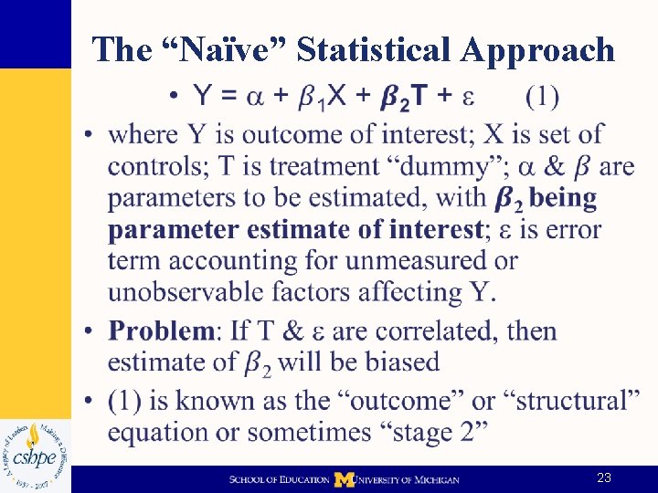
The “Naïve” Statistical Approach • 23

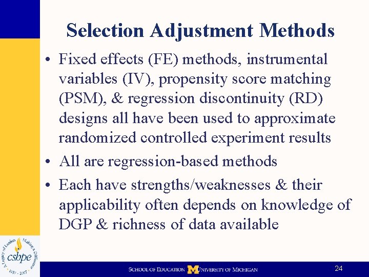
Selection Adjustment Methods • Fixed effects (FE) methods, instrumental variables (IV), propensity score matching (PSM), & regression discontinuity (RD) designs all have been used to approximate randomized controlled experiment results • All are regression-based methods • Each have strengths/weaknesses & their applicability often depends on knowledge of DGP & richness of data available 24

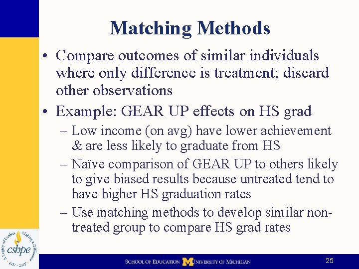
Matching Methods • Compare outcomes of similar individuals where only difference is treatment; discard other observations • Example: GEAR UP effects on HS grad – Low income (on avg) have lower achievement & are less likely to graduate from HS – Naïve comparison of GEAR UP to others likely to give biased results because untreated tend to have higher HS graduation rates – Use matching methods to develop similar nontreated group to compare HS grad rates 25

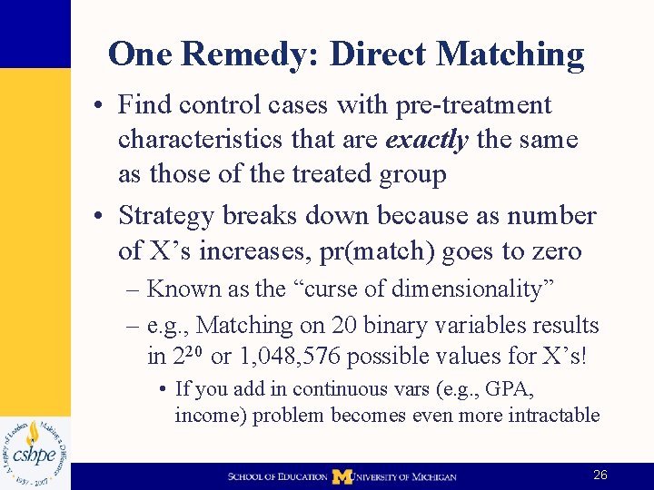
One Remedy: Direct Matching • Find control cases with pre-treatment characteristics that are exactly the same as those of the treated group • Strategy breaks down because as number of X’s increases, pr(match) goes to zero – Known as the “curse of dimensionality” – e. g. , Matching on 20 binary variables results in 220 or 1, 048, 576 possible values for X’s! • If you add in continuous vars (e. g. , GPA, income) problem becomes even more intractable 26

Propensity Score Matching • Solution: Estimate the “propensity score” (PS) & match treated with control cases based only on this single number – This approach controls for pre-treatment differences by balancing each group’s set of observable characteristics on a single number • Goal: Estimate treatment effects for individuals with similar observable characteristics, as indexed by the PS 27

Estimating the Propensity Score • Estimate Pr(treatment) – Typically done using logistic regression, but some software uses probit • Use PS to find control(s) with “same” score as treated observation – Establishes counterfactual (“control” group) • Test for differences in outcomes between treated & counterfactual (“controls”) – Often done using regression methods 28

Goal of PS Matching • When done correctly, probability that treated observation has specific trait (X=x) is same as Pr(untreated) has (X=x) • PSM is basically a “resampling” or even “oversampling” method, which involves a bias & variance tradeoff – e. g. , When matching with replacement, avg. match quality increases & bias decreases, but fewer distinct controls are used, increasing the variance of the estimator 29

PSM Assumptions: Conditional Independence Assumption • Conditional on observables, there is no correlation between the treatment & outcome that occurs absent the treatment Mathematically: (Y 1 , Y 0 ) ┴ D | X • After controlling for observables, the treatment assignment is as good as random • Upshot: Untreated observations can serve as the counterfactual for the treated 30

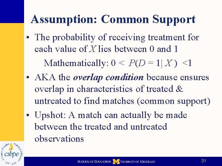
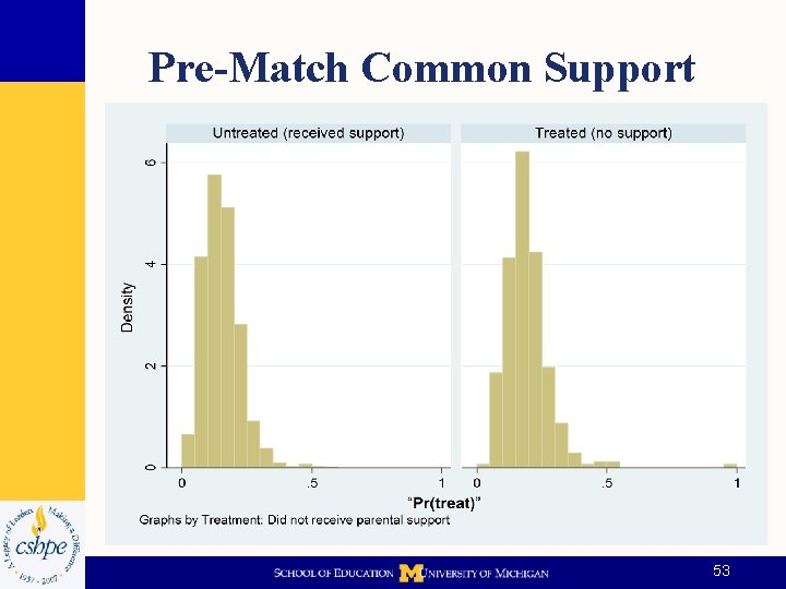
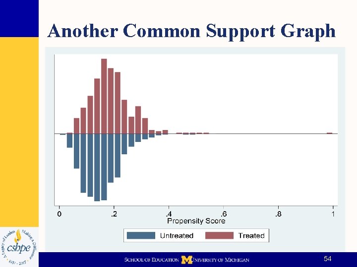
Assumption: Common Support • The probability of receiving treatment for each value of X lies between 0 and 1 Mathematically: 0 < P(D = 1| X ) <1 • AKA the overlap condition because ensures overlap in characteristics of treated & untreated to find matches (common support) • Upshot: A match can actually be made between the treated and untreated observations 31

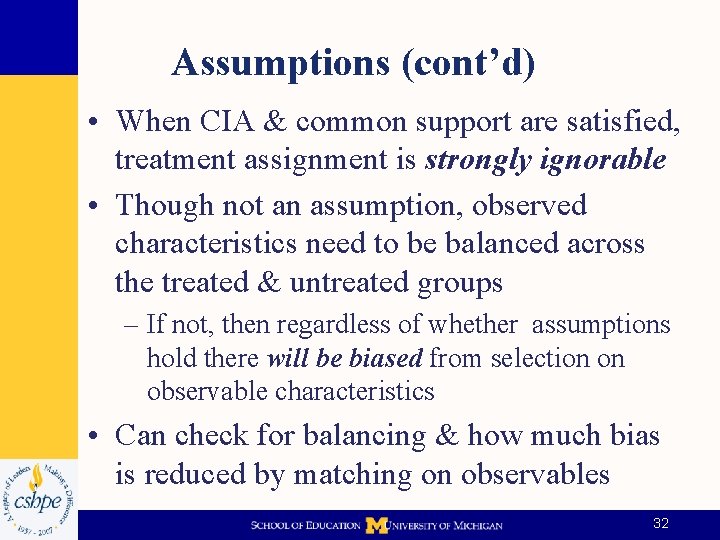
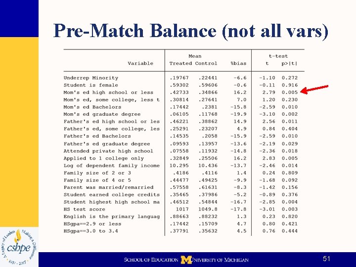
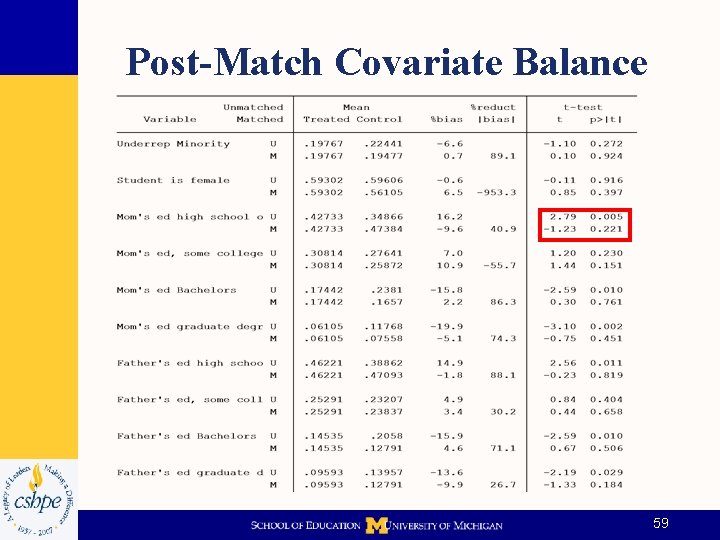
Assumptions (cont’d) • When CIA & common support are satisfied, treatment assignment is strongly ignorable • Though not an assumption, observed characteristics need to be balanced across the treated & untreated groups – If not, then regardless of whether assumptions hold there will be biased from selection on observable characteristics • Can check for balancing & how much bias is reduced by matching on observables 32

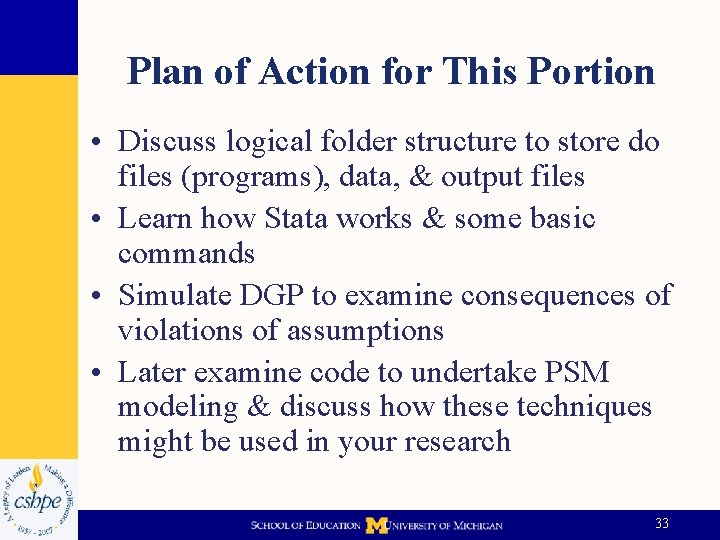
Plan of Action for This Portion • Discuss logical folder structure to store do files (programs), data, & output files • Learn how Stata works & some basic commands • Simulate DGP to examine consequences of violations of assumptions • Later examine code to undertake PSM modeling & discuss how these techniques might be used in your research 33

Importance of Good Structure • My bet is that IR folks like you know this already but… • Creating a logical folder structure for each project is important step in analysis process • If you use a similar structure all the time you will be able to come back to projects at later date & understand what was done • Also very important to provide comments in your do files so you know what you did – Maybe someone else will pick up your work 34

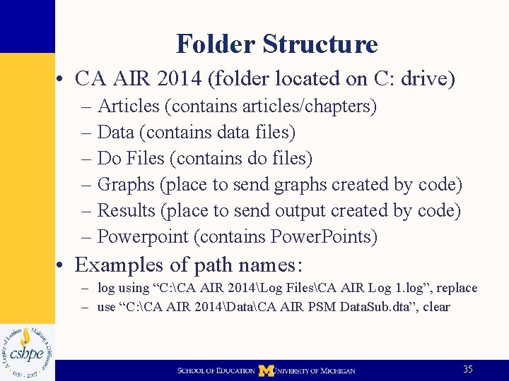
Folder Structure • CA AIR 2014 (folder located on C: drive) – Articles (contains articles/chapters) – Data (contains data files) – Do Files (contains do files) – Graphs (place to send graphs created by code) – Results (place to send output created by code) – Powerpoint (contains Power. Points) • Examples of path names: – log using “C: CA AIR 2014Log FilesCA AIR Log 1. log”, replace – use “C: CA AIR 2014DataCA AIR PSM Data. Sub. dta”, clear 35

How Stata Works • Command or “point & click” driven software • Software resides in: – C: Program Files (x 86) Stata 13 (or Stata 12) – Type: “adopath” on command line to find paths to the ado files used • Role of “ado” files – Examine ado & help files • Discuss user written ado & help files 36

The “Look” of Stata • Toolbar contains icons that allow you to Open & Save files, Print results, control Logs, & manipulate windows • Of particular interest: Opening the Do-File Editor, the Data Editor and the Data Browser. – Data Editor & Browser: Spreadsheet view of data • Do-File Editor allows you to construct a file of Stata commands, save them, & execute all/parts • The Current Working Directory is where any files created in your active Stata session will be saved (by default). – Don’t save stuff here, direct to folders discussed above 37

Windows in Stata • Review, Results, Command, & Variables windows • Help: Search for any command/feature. Help Browser, which opens in Viewer window, provides hyperlinks to help pages & to pages in the Stata manuals (which are quite good) • May search for help using command line • Role of “findit” & “ssc install” – Locate commands in Stata Technical Bulletin & Stata Journal; Demo loading the “psmatch 2” command – On command line type: “ssc describe psmatch 2” then “ssc install psmatch 2” & then “help psmatch 2” 38

Stata Program Files • Called “do” files; contain Stata code/commands we “run” to produce results • Do File Name: – CA AIR PSM Violations Simulation. do in the “Do Files” sub-folder in CA AIR 2014 main project folder – Later will use: CA AIR PSM. do in same place • There also menu options to run commands in Stata, but we won’t do this – May be useful for some “on the fly” analysis, but it is NOT a good way to do most projects – Reasons: Reproducibility & transportability 39

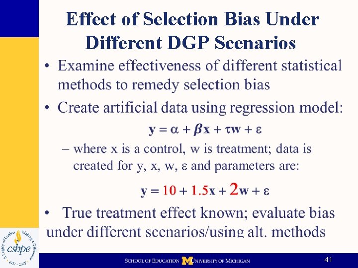
Simulating Condition Violations • Before delving into real application of propensity score matching in education research, we will examine effects of a few condition/assumption violations on results • To do so, we’ll create “fake” data set so we know true parameters & can therefore figure out bias due to such violations 40

Effect of Selection Bias Under Different DGP Scenarios • 41

Simulations Conducted • Relax following conditions: – No correlation between x and e – No correlation between x and w 42

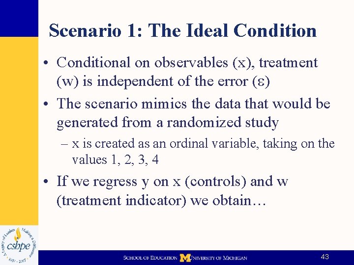
Scenario 1: The Ideal Condition • Conditional on observables (x), treatment (w) is independent of the error (e) • The scenario mimics the data that would be generated from a randomized study – x is created as an ordinal variable, taking on the values 1, 2, 3, 4 • If we regress y on x (controls) and w (treatment indicator) we obtain… 43

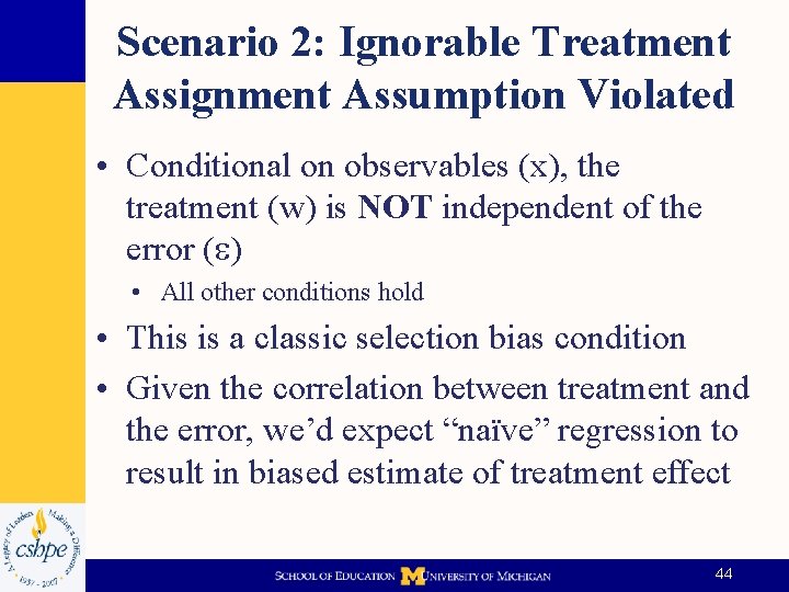
Scenario 2: Ignorable Treatment Assignment Assumption Violated • Conditional on observables (x), the treatment (w) is NOT independent of the error (e) • All other conditions hold • This is a classic selection bias condition • Given the correlation between treatment and the error, we’d expect “naïve” regression to result in biased estimate of treatment effect 44

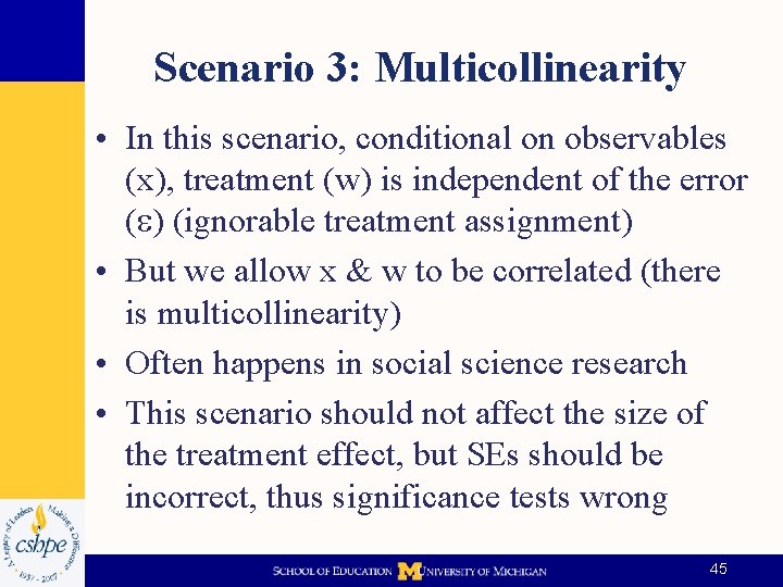
Scenario 3: Multicollinearity • In this scenario, conditional on observables (x), treatment (w) is independent of the error (e) (ignorable treatment assignment) • But we allow x & w to be correlated (there is multicollinearity) • Often happens in social science research • This scenario should not affect the size of the treatment effect, but SEs should be incorrect, thus significance tests wrong 45

Scenario 4 • There is correlation between the regressors and non-ignorable treatment assignment • Correlation between x and error & t • x is continuous instead of ordinal • All other assumptions from Scenario 1 hold • Pattern in graph is produced by correlation between treatment & error term • Happens when control variables (x’s) are omitted • Known as "selection on unobservables" 46

Scenario 5 • In this scenario t and x correlated with the error term; w and x are also correlated • This scenario assumes the weakest conditions for data generation • The results produced by both the naïve regression and the matching methods result in substantial bias in the estimation of the treatment effect 47

Does Failure of Parents to Provide Required Support Hinder Student Success? • Some parents provide the support they are required to, others do not • Inferential problem: Students who do not get support (“treated”) may be different (on observed & unobserved factors) than those who receive support – Correlation between Pr(no support) & educational outcomes makes parsing causal effects from observed & unobserved differences in students very difficult 48

Empirical Example • Examine whether lack of expected parental financial support causes differences in: – Loan use; attending part-time; worked 20+ hours/week in college; whether student dropped out in year one; completion of a bachelor’s degree within 6 years • Treatment variable: T = 1 if student did not receive required funds from their parents to pay for college expenses; 0 otherwise 49

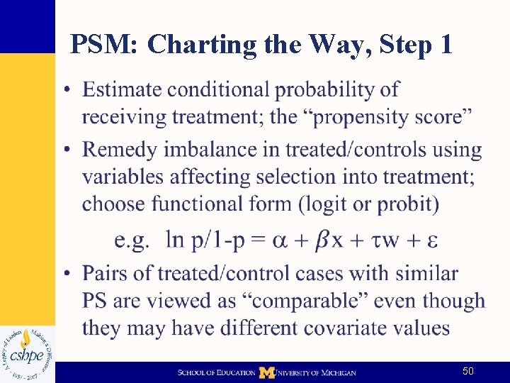
PSM: Charting the Way, Step 1 • 50

Pre-Match Balance (not all vars) 51

Step 2: Matching • Propensity score used to match treated to control case(s) to make cases “alike” • Extent of “common support” will dictate whethere is match for all treated – Lack of will lead to non-matches; loss of cases • Thus, this is really resampling, with new sample balanced in terms of selection bias • Many algorithms available to match cases with similar PS 52

Pre-Match Common Support 53

Another Common Support Graph 54

Variable Selection • May want to include large # of variables & remove insignificant ones • May improve fit according to model fit measures, but does not focus on the task at hand: Achieving balance among Xs (satisfying the CIA). • An X may not be significant but removing it may remove important variation necessary to satisfy CIA. 55

Variable Selection (cont’d) • Use conceptual theory & prior research to suggest necessary conditioning Xs • Xs affecting selection into treatment & the outcome can and should be included • Need to be careful about temporal ordering – Only variables unaffected by participation (or the anticipation of it) should be included • Some debate in literature about specification of PS regression model 56

Step 3: Post-Matching Analysis • Balanced sample corrects for selection bias & violations of assumptions inherent when using naïve statistical methods to est. effects • Use resample to do multivariate analysis as normally would if DGP from randomization – Could also stratify on PS and compare means between treated/controls in each stratum • Many variations on this general 3 step approach; see Guo & Fraser for details 57

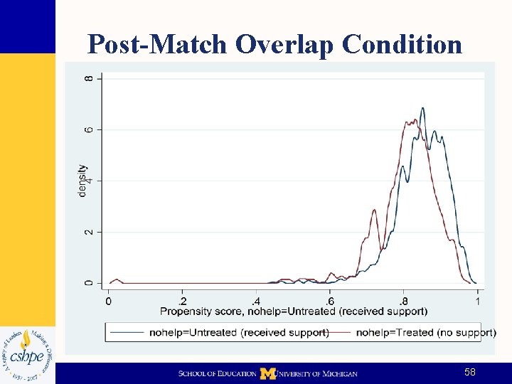
Post-Match Overlap Condition 58

Post-Match Covariate Balance 59

Different Matching Algorithms • Nearest Neighbor: Treated obs matched to control obs with similar PS – Latter case used as counterfactual former • Can perform NN with/without replacement – With: Higher quality matches (< biased) by always using closest neighbor regardless of whether it has been used before • Doing so increases variance of estimates because fewer untreated units are used in the matching 60

Matching Algorithms (cont’d) – Without replacement: Order in which matches made is important because matches must be unique. If made in particular order (going from low to higher PS), then systematic biases may be built in. – When using NN matching without replacement it is critical that order in which the matches are made be random. • Will see how to do this later 61

Caliper & Radius Matching • Drawback of NN: NN may not be near! • Caliper matching: NN & define range in which acceptable matches can be made – Bandwidth chosen by researcher; represents max interval in which to make a match – NN outside of bandwidth, no match & treated case has no counterfactual/not used – Method imposes common support for each observation in the data 62

Caliper & Radius (cont’d) • Caliper: Treated obs PS =. 40 & h=. 05 – Where h is the “bandwidth” Match made if 0. 35<= NN <= 0. 45. • Equivalent when matching with replacement is called “radius” matching – Matches within bandwidth are equally weighted when constructing counterfactual • Both require h & bias/Var tradeoff – Wider h lowers Var as more data used, but also lowers the match quality & bias increases 63

Kernel & Local Linear Regression • Both are one-to-many algorithms • Unlike radius, these weight each untreated obs according to how close match is • Function determining weight: the “kernel” – As match becomes worse; weight on untreated unit decreases • LLR uses kernel to weight obs but does so using regression-based methods • Both are computationally intensive 64

PS Reweighting • Simpler procedure focuses on reweighting & does not involve matching obs – AKA “inverse probability weighting” • Reweight untreated obs with high (low) PS up (down) – Untreated obs with high PS most like treated so weight more heavily than the observations that are dissimilar (as indicated by low PS) – Advantage: Program ease because no need to create counterfactuals for each unit one-by-one. 65

Inference • How to construct SEs of treatment effects? • Incorrect to t-test on null ATT=0; doesn’t account for V intro. by estimation of PS • Solution: Use teffects command or if using psmatch 2 need to bootstrap SEs to obtain correct CIs for estimated effects • Randomly pull obs (with replacement) then calc. effect; draw new sample; est another effect; do this many (e. g. , thousands) times 66

Inference (cont’d) • For NN using psmatch 2, bs may not produce accurate SEs – Lack of “smoothness” of algorithm? • Smoother algorithms, such as kernel matching, local linear regression, & PS reweighting may not suffer from similar problems • Despite concerns, bs is most common method for producing SEs in matching methods (if not using teffects command) 67

Bounding • If there are unobserved variables that simultaneously affect assignment into treatment & the outcome variable, a hidden bias might arise to which matching estimators are not robust • Since estimating the magnitude of selection bias with nonexperimental data is not possible, we address this problem with the bounding approach proposed by Rosenbaum (2002) 68

Bounding • The basic question is whether unobserved factors can alter inference about treatment effects. One wants to determine how strongly an unmeasured variable must influence the selection process to undermine the implications of the matching analysis. • Rbounds test sensitivity for continuousoutcome variables, mhbounds for binaryoutcome variables 69

Bounding • if there is hidden bias, two individuals with the same observed covariates x have different chances of receiving treatment • Sensitivity analysis now evaluates how changing the values of γ and (ui−uj) alters inference about the program effect. • individuals who appear to be similar (in terms of x) could differ in their odds of receiving the treatment by as much as a factor of 2. In this sense, eγ is a measure of 70 the degree of departure from a study that is

Pros/Cons of PSM • Benefits – Make inference from comparable group – Focuses on population of interest – Use of propensity score solves the dimensionality problem in direct matching • Limitations – Cannot directly control for unobserved characteristics that affect the outcome • Can, however, examine sensitivity of this, which is an innovation in method 71

Conclusions • RCTs are desirable in terms of making causal statements, but often difficult to employ • In education we often have observational data but methods used to make statements of treatment effects are typically deficient • Ultimate goal: Make strong (“causal”) statements to improve knowledge of mechanisms that determine program & practice effectiveness • We need to be much more attentive to the problems that arise when we are using observational data 72

Other Take Aways • Education research has not kept pace with advances in quantitative methods • There are really few good reasons for not applying these new methods • There is a payoff for doing so: Better information about the mechanisms that affect higher education processes, policies, and outcomes • We need to employ these methods more broadly in IR to ascertain “what works” 73

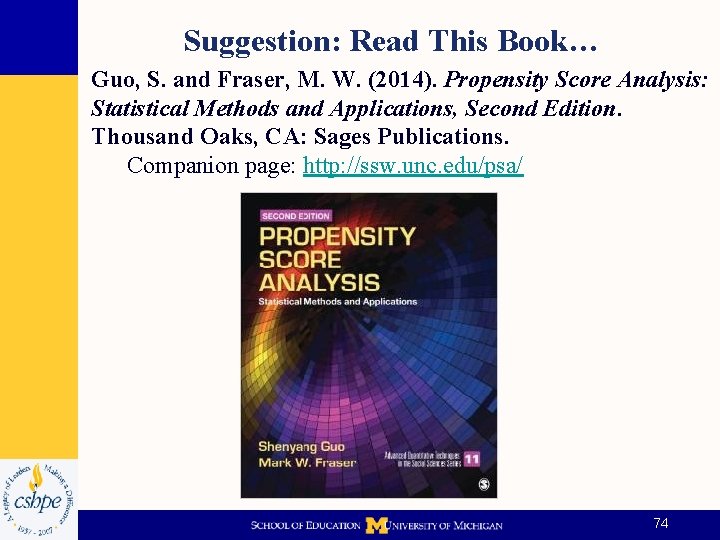
Suggestion: Read This Book… Guo, S. and Fraser, M. W. (2014). Propensity Score Analysis: Statistical Methods and Applications, Second Edition. Thousand Oaks, CA: Sages Publications. Companion page: http: //ssw. unc. edu/psa/ 74

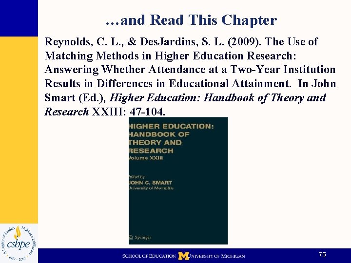
…and Read This Chapter Reynolds, C. L. , & Des. Jardins, S. L. (2009). The Use of Matching Methods in Higher Education Research: Answering Whether Attendance at a Two-Year Institution Results in Differences in Educational Attainment. In John Smart (Ed. ), Higher Education: Handbook of Theory and Research XXIII: 47 -104. 75

Purchasing Stata • Depending on your needs, there a number of software options when purchasing Stata • Single user/institutional/Grad Plan licenses • Small vs. IC vs. SE versions • Perpetual license; continually updated • Stat Transfer software • See the Stata website for more information: http: //www. stata. com/order/educational-purchases/dl/ 76

References • • • Adelman, C. (1999). Answers in the toolbox: Academic intensity, attendance patterns, and bachelor‘s degree attainment. Washington, D. C. : U. S. Department of Education. Adelman, C. (2006). The toolbox revisited: Paths to degree completion from high school through college. Washington, D. C. : U. S. Department of Education. Angrist, J. D. , & Pischke, J. S. (2009). Mostly harmless econometrics. Princeton, NJ: Princeton University Press. Caliendo, M. & Kopeinig, S. (2008) Some practical guidance for the implementation of propensity score matching. Journal of Economic Surveys, 22, 31 -72. Cohn, E. , & Geske, T. G. (1990). The economics of education (3 rd ed. ). Oxford: Pergamon Press. Guo, S. and Fraser, M. W. (2010). Propensity Score Analysis: Statistical Methods and Applications. Thousand Oaks, CA: Sages Publications. – Companion page: http: //ssw. unc. edu/psa/ Holland, P. W. (1986). Statistics and causal inference. Journal of the American Statistical Association, 81(396), 945– 960. Heckman J. J. (1976). The common structure of statistical models of truncation, sample selection and limited dependent variables and a simple estimator for such models. Annals of Economic and Social Measurement, 5, 475– 492. Heckman, J. J. (1979). Sample selection bias as a specification error. Econometrica, 47(1), 153– 161. 77

References • • • Mincer, J. (1958). Investment in human capital and personal income distribution. Journal of Political Economy, 66(4), 281 -302. Morgan, S. L. and Winship, C. (2007). Counterfactuals and Causal Inference: Methods and Principles for Social Research. Cambridge, UK: Cambridge University Press. Reynolds, C. L. , & Des. Jardins, S. L. (2009). The Use of Matching Methods in Higher Education Research: Answering Whether Attendance at a Two-Year Institution Results in Differences in Educational Attainment. In John Smart (Ed. ), Higher Education: Handbook of Theory and Research XXIII: 47 -104. Rose, H. , & Betts, J. R. (2001). Math matters: The links between high school curriculum, college graduation, and earnings. San Francisco, CA: Public Policy Institute of California. Rosenbaum, P. R. , & Rubin, D. B. (1985). Constructing a Control Group Using Multivariate Matched Sampling Methods That Incorporate the Propensity Score. The American Statistician, 39(1), 33 -38. Rosenbaum, P. R. (2002). Observational Studies. 2 nd ed. New York: Springer. Rosenbaum, P. R. (2010). Design of observational studies. New York: Springer Rubin, D. B. (1974). Estimating causal effects of treatments in randomized and nonrandomized studies. Journal of Educational Psychology, 66(5), 688– 701. Rubin, D. B. (1977). Assignment of treatment group on the basis of a covariate. Journal of Educational Statistics, 2, 1– 26. 78

References • • • Rubin, D. B. (1978). Bayesian inference for causal effects: The role of randomization. Annals of Statistics, 6, 34– 58. Rubin, D. B. (1980). Discussion of “Randomization analysis of experimental data in the Fisher randomization test” by Basu. Journal of the American Statistical Association, 75, 591– 593. Schneider, B. , Carnoy, M. , Kilpatrick, J. , Schmidt, W. H. , & Shavelson, R. J. (2007). Estimating Causal Effects Using Experimental and Observational Designs. Washington, DC: American Educational Research Association. Shadish, W. R. , Cook, T. D. , Campbell, D. T. (2002). Experimental and quasiexperimental designs for generalized causal inference. Boston: Houghton-Mifflin Stuart, E. A. (2010) Matching methods for causal inference: A review and a look forward. Statistical Science, 25(1), 1 -21. 79

• Thank You for Your Kind Attention! 80

Background Material

Recent AERA Report on the Issue • “Recently, questions of causality have been at the forefront of educational debates and discussions, in part because of dissatisfaction with the quality of education research…”. A common concern “revolves around the design of and methods used in education research, which many claim have resulted in fragmented and often unreliable findings” (Schneider, et al. , 2007) 82

Definition of Cause and Effect • “A cause is that which makes any other thing, either simple idea, substance, or mode, begin to be; and an effect is that which had its beginning from some other thing” (Locke, 1690/1975, p. 325). 83

Holding • In quintiles, you divide your sample into five groups, the 20% LEAST likely to end up in your treatment group is quintile 1, the 20% with the GREATEST likelihood of ending up in your treatment group is quintile 5, and so on. You match the subjects by quintiles. So, if 12% of the treatment group is in quintile 1, you randomly select 12% of the control subjects from quintile 1. In nearest neighbor matching, as the name implies, you match each subject in the treatment group with a subject in the control group who is nearest in probability of ending up in the treatment group. Then, there is the calipers (radius) matching, that uses the nearest neighbors within a given radius or interval. ESSENTIAL REFERENCES Propensity score matching Rosenbaum, P. R. and Rubin, D. B. (1983), “The Central Role of the Propensity Score in Observational Studies for Causal Effects”, Biometrika, 70, 1, 41 -55. Caliper matching Cochran, W. and Rubin, D. B. (1973), “Controlling Bias in Observational Studies”, Sankyha, 35, 417 -446. Kernel-based matching Heckman, J. J. , Ichimura, H. and Todd, P. E. (1997), “Matching As An Econometric Evaluation Estimator: Evidence from Evaluating a Job Training Programme”, Review of Economic Studies, 64, 605 -654. Heckman, J. J. , Ichimura, H. and Todd, P. E. (1998), “Matching as an Econometric Evaluation Estimator”, Review of Economic Studies, 65, 261 -294. Mahalanobis distance matching Rubin, D. B. (1980), “Bias Reduction Using Mahalanobis-Metric Matching”, Biometrics, 36, 293 -298. 84

Data Set Used • Data Set Name: CA AIR PSM Data. Sub. dta that is located in the “Data” sub-folder in the CA AIR 2014 main project folder • The data contains a subset of national education data – Only select variables are included in the dataset 85

Summary • These methods, and others, can be helpful in studying the effects of programs, process, & practices where random assignment is not possible or feasible. • They are regression-based so learning them is an extension of the OLS/logit training many have had • The results can be displayed in a way so as to make them understandable to policy makers & administrators 86

Summary (cont’d) • There are many resources available to learn & extend these methods – Higher education literature, Stata (and other) publications, blogs with code & solutions to programming/statistical problems – Professional development workshops • I hope you’ve found this exercise helpful & that you will be able to use these methods in your IR work 87