Matching Procedures Propensity Score Hctor Lamadrid Center for

Matching Procedures: Propensity Score Héctor Lamadrid Center for Population Health Research National Institute of Public Health, Mexico

What is matching for? § In an ideal setting, we will always have a random assignment of the treatment. § This makes estimating the programme effect straightforward and relativley easy… § However: Often this is not possible, or we are called to evaluate once the programme is running… § What to do? We always need to look for the best possible proxy of the counterfactual

Matching § Suppose that individuals are voluntarily enrolling (or not enrolling) in a programme. § It is very likely that those who decide to enroll are very different to those who don’t § A simple comparison between both groups will surely be very biased.

Matching § What to do then? § Take one subject A, who enrolled…. § Look for other subject who is almost identical to subject A, but who DID NOT ENROLL, lets call him subject B. He will be our proxy of the counterfactual § Calculate the difference in the outcome between both subjects. § Repeat for all the treated subjects… § Voilá! We get an estimate of the Average Treatment Effect!

Matching § All this sounds great but note that subject B must be almost identical to A, that means we desire both to have the exact same values of MANY variables related to the outcome.

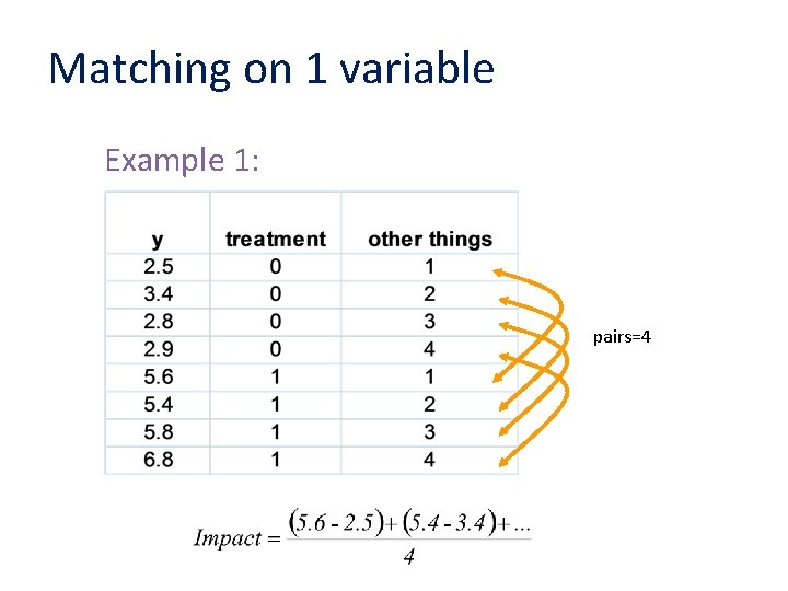
Matching on 1 variable Example 1: pairs=4

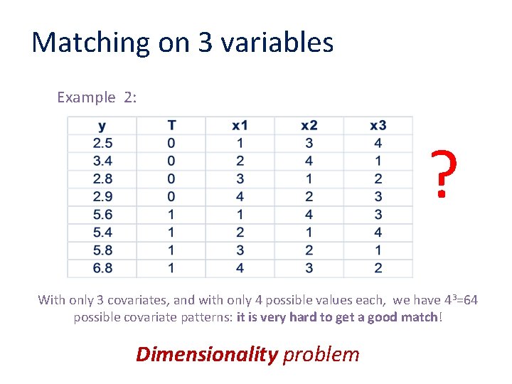
Matching on 3 variables Example 2: ? With only 3 covariates, and with only 4 possible values each, we have 43=64 possible covariate patterns: it is very hard to get a good match! Dimensionality problem

Matching § So we could try to match on several important variables but adding more variables makes it exponentially more difficult to find a match. § So… Rosenbaum & Rubin came up with this idea of collapsing all information of covariates in a single measure: § The “Propensity Score”

The propensity score § Employs a predicted probability of group membership—e. g. , treatment vs. control group-based on observed predictors, usually obtained from logistic or probit regression to create a counterfactual proxy. § Propensity scores may be used for matching or as covariates in a regression model—alone or with other matching variables or covariates.

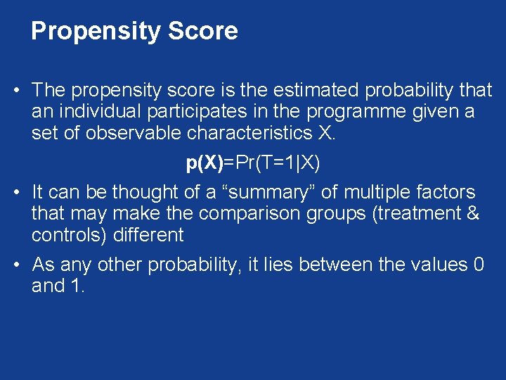
Propensity Score • The propensity score is the estimated probability that an individual participates in the programme given a set of observable characteristics X. p(X)=Pr(T=1|X) • It can be thought of a “summary” of multiple factors that may make the comparison groups (treatment & controls) different • As any other probability, it lies between the values 0 and 1.

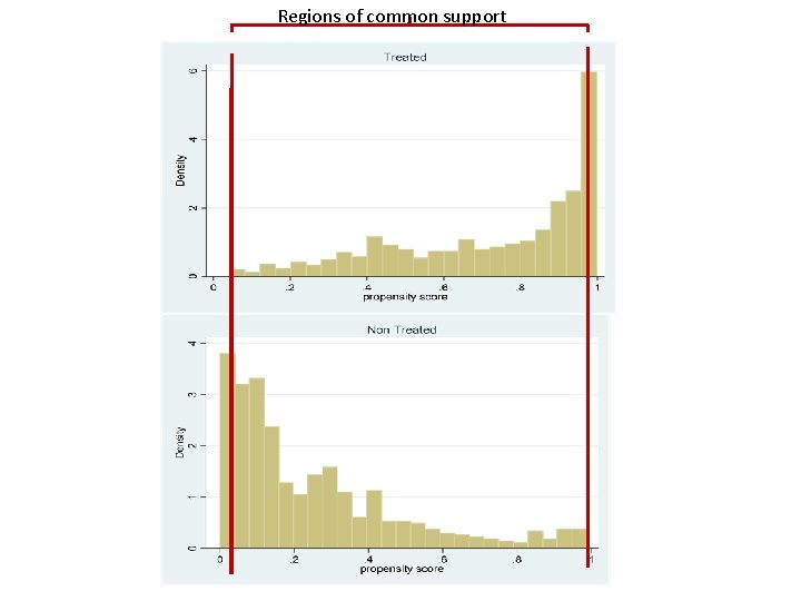
Propensity Score • Useful for matching: Instead of matching on an enormous set of covariates, we can match two individuals who have the same probability of being enrolled in the programme! • We have to make a couple of important assumptions: • Conditional on X, the treatment assignment is independent of the potential outcomes. • There is a common support area (an overlap of the distribution of p(X) in the treatment & control groups)

Regions of common support

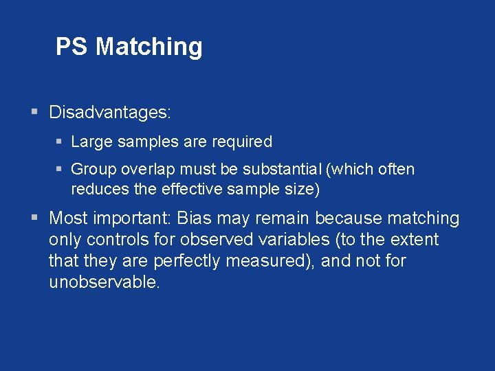
PS Matching § Disadvantages: § Large samples are required § Group overlap must be substantial (which often reduces the effective sample size) § Most important: Bias may remain because matching only controls for observed variables (to the extent that they are perfectly measured), and not for unobservable.

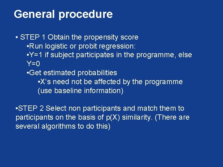
General procedure • STEP 1 Obtain the propensity score • Run logistic or probit regression: • Y=1 if subject participates in the programme, else Y=0 • Get estimated probabilities • X’s need not be affected by the programme (use baseline information) • STEP 2 Select non participants and match them to participants on the basis of p(X) similarity. (There are several algorithms to do this)

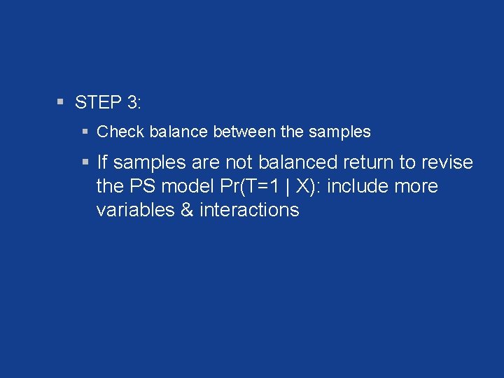
§ STEP 3: § Check balance between the samples § If samples are not balanced return to revise the PS model Pr(T=1 | X): include more variables & interactions

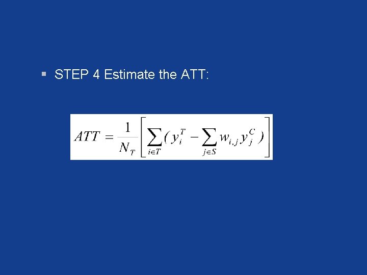
§ STEP 4 Estimate the ATT:

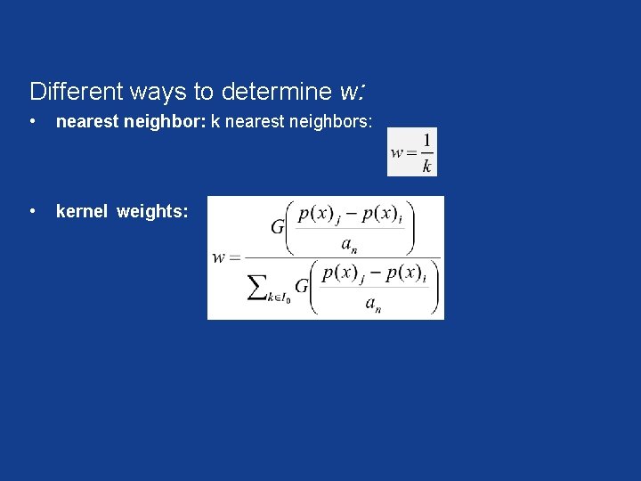
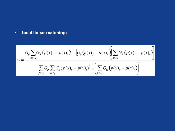
Different ways to determine w: • nearest neighbor: k nearest neighbors: • kernel weights:

• local linear matching:

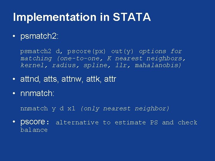
Implementation in STATA • psmatch 2: psmatch 2 d, pscore(px) out(y) options for matching (one-to-one, K nearest neighbors, kernel, radius, spline, llr, mahalanobis) • attnd, atts, attnw, attk, attr • nnmatch: nnmatch y d x 1 (only nearest neighbor) • pscore: balance alternative to estimate PS and check

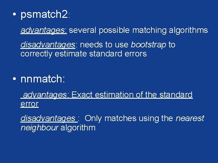
• psmatch 2: advantages: several possible matching algorithms disadvantages: needs to use bootstrap to correctly estimate standard errors • nnmatch: advantages: Exact estimation of the standard error disadvantages : Only matches using the nearest neighbour algorithm

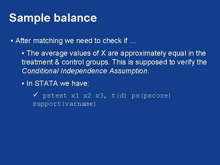
Sample balance • After matching we need to check if … • The average values of X are approximately equal in the treatment & control groups. This is supposed to verify the Conditional Independence Assumption. • In STATA we have: ü pstest x 1 x 2 x 3, t(d) ps(pscore) support(varname)

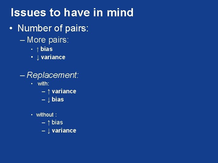
Issues to have in mind • Number of pairs: – More pairs: • ↑ bias • ↓ variance – Replacement: • with: – ↑ variance – ↓ bias • without : – ↑ bias – ↓ variance

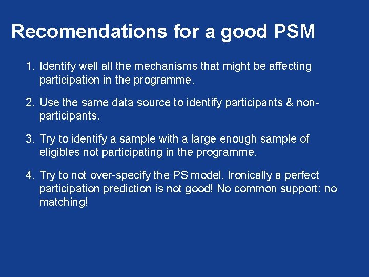
Recomendations for a good PSM 1. Identify well all the mechanisms that might be affecting participation in the programme. 2. Use the same data source to identify participants & nonparticipants. 3. Try to identify a sample with a large enough sample of eligibles not participating in the programme. 4. Try to not over-specify the PS model. Ironically a perfect participation prediction is not good! No common support: no matching!

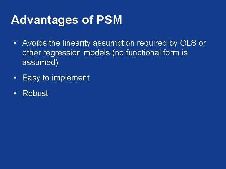
Advantages of PSM • Avoids the linearity assumption required by OLS or other regression models (no functional form is assumed). • Easy to implement • Robust

Disadvantages • Does not deal with unobservables • Requires a common support: • No common support, no matching • Requires a lot of information to model the participation process