Patterns in Evolution I Phylogenetic II Morphological III

Patterns in Evolution I. Phylogenetic II. Morphological III. Historical (later) IV. Biogeographical

Patterns in Evolution I. Phylogenetic - Determining the genealogical, familial patterns among organisms, populations, species and higher taxa - "family trees"

Patterns in Evolution I. Phylogenetic A. Systematics: Taxonomy and Classification

Patterns in Evolution I. Phylogenetic A. Systematics: Taxonomy and Classification 1. Taxonomy - the naming of taxa (singular 'taxon")

Patterns in Evolution I. Phylogenetic A. Systematics: Taxonomy and Classification 1. Taxonomy - the naming of taxa (singular 'taxon") a. Rules for naming species: • Latin binomen (Drosophila melanogaster) • italicized or underlined • author recognized in some groups (insects) • Genus - species agree in gender • unambiguous within a kingdom • if a species is named twice, priority counts • based on a 'holotype' or 'type' specimen • 'paratypes' show range of variation • 'species' is both singular and plural; genus (s. ), genera (pl. )

Patterns in Evolution I. Phylogenetic A. Systematics: Taxonomy and Classification 1. Taxonomy - the naming of taxa (singular 'taxon") b. Rules for renaming species • if assigned to new genus, epithet stays • new author name placed in parens

Patterns in Evolution I. Phylogenetic A. Systematics: Taxonomy and Classification 1. Taxonomy - the naming of taxa (singular 'taxon") c. Rules for higher taxa • Animal families end in "-idae" (Felidae) • Animal sub-families end in "-inae" (Homininae) • These are often derived from the same stem as the 'type genus' the first genus described for the family. (Felis) • Plant families end in "-aceae" (Betulaceae) • Higher taxa are capitalized, but not italicized (as above) • adjectives are not capitalized ("hominids")

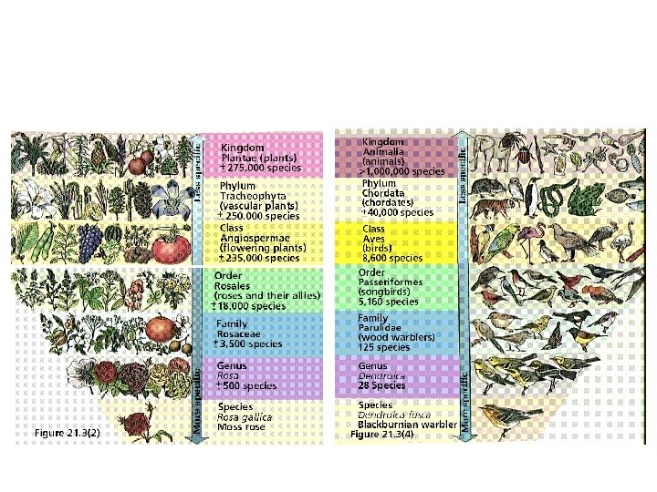
Patterns in Evolution I. Phylogenetic A. Systematics: Taxonomy and Classification 1. Taxonomy - the naming of taxa (singular 'taxon") 2. Classification - determining the hierarchical position of each species within higher taxa. a. The Hierarchy. .

Patterns in Evolution I. Phylogenetic A. Systematics: Taxonomy and Classification 1. Taxonomy - the naming of taxa (singular 'taxon") 2. Classification - determining the hierarchical position of each species within higher taxa. a. The Hierarchy. . b. Issues

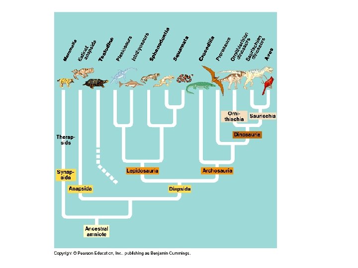
Patterns in Evolution I. Phylogenetic A. Systematics: Taxonomy and Classification 1. Taxonomy - the naming of taxa (singular 'taxon") 2. Classification - determining the hierarchical position of each species within higher taxa. a. The Hierarchy. . b. Issues • Cladogenesis: you want the branching/"clade" pattern of taxa to reflect phylogenetic relationships – “Archosaurs” for crocodilians and birds…

Patterns in Evolution I. Phylogenetic A. Systematics: Taxonomy and Classification 1. Taxonomy - the naming of taxa (singular 'taxon") 2. Classification - determining the hierarchical position of each species within higher taxa. a. The Hierarchy. . b. Issues • Cladogenesis: you want the branching/"clade" pattern of taxa to reflect phylogenetic relationships – “Archosaurs” for crocodilians and birds… • Anagenesis: however, some evolutionary changes are so profound that we might honor the degree of difference ("Class: Aves”)

c. Terms: Monophyletic taxon: includes all (and only) the species descended from a common ancestor. Aves is good.

c. Terms: Monophyletic taxon: includes all (and only) the species descended from a common ancestor. Aves is good. Paraphyletic taxon: includes all descendants of a common ancestor, except for those placed in another taxon. So, “Reptilia” is a paraphyletic group, as it includes all diapsids and anapsids EXCEPT birds. OR, it includes all amniotes EXCEPT mammals and birds (this gets the synapsids).

c. Terms: Monophyletic taxon: includes all (and only) the species descended from a common ancestor. Aves is good. Paraphyletic taxon: includes all descendants of a common ancestor, except for those placed in another taxon. So, “Reptilia” is a paraphyletic group, as it includes all diapsids and anapsids EXCEPT birds. OR, it includes all amniotes EXCEPT mammals and birds (this gets the synapsids). Polyphyletic taxon: includes organisms that do not share a common ancestor that is in the group. To be avoided. “Fliers” (Birds, Pterosaurs)

Patterns in Evolution I. Phylogenetic A. Systematics: Taxonomy and Classification 1. Taxonomy - the naming of taxa (singular 'taxon") 2. Classification - determining the hierarchical position of each species within higher taxa. a. The Hierarchy. . b. Issues c. Terms: d. Philosophy of Cladistics: • Term coined by Willi Hennig suggested that classification should only include monophyletic groups, and that phylogeny should be inferred from the analyses of shared derived traits. • This gives strong preference to cladogenesis over anagenesis, such that ‘birds’ really be classified as a derived group of dinosaurs or reptiles, not as “separate” from them. http: //palaeos. com/vertebrates/theropoda/dinosaurs-birds. html

Linnaean Classification of Apes Hominidae Pongidae Hylobatidae Apes = primates (grasping hands, binocular vision) with no tails

Linnaean Classification of Apes Hylobatidae Pongidae PARAPHYLETIC

Linnaean Classification of Apes Hylobatidae Hominidae

Patterns in Evolution I. Phylogenetic A. Systematics: Taxonomy and Classification B. Reconstructing Phylogenies

Patterns in Evolution I. Phylogenetic A. Systematics: Taxonomy and Classification B. Reconstructing Phylogenies 1. Characters • morphological • behavioral • cellular (structural or chemical) • genetic - nitrogenous base sequence; amino acid sequence

Patterns in Evolution I. Phylogenetic A. Systematics: Taxonomy and Classification B. Reconstructing Phylogenies 1. Characters • morphological • behavioral • cellular (structural or chemical) • genetic - nitrogenous base sequence; amino acid sequence • can be quantitative measurements, or qualitative "presence/absence"

Patterns in Evolution I. Phylogenetic A. Systematics: Taxonomy and Classification B. Reconstructing Phylogenies 1. Characters 2. Trees a. Unrooted trees: show patterns among groups without specifying ancestral relationships Trait 1 Trait 2 Trait 3 Trait 4 Trait 5 A 0 0 0 1 1 B 0 0 1 1 1 C 1 1 1 0 1 D 1 1 0 0 1

Patterns in Evolution I. Phylogenetic A. Systematics: Taxonomy and Classification B. Reconstructing Phylogenies 1. Characters 2. Trees So, A and B share three traits that C and D don't have (1, 2, 4) and are more similar to one another than they are to C and D. Trait 1 Trait 2 Trait 3 Trait 4 Trait 5 A 0 0 0 1 1 B 0 0 1 1 1 C 1 1 1 0 1 D 1 1 0 0 1

Patterns in Evolution I. Phylogenetic A. Systematics: Taxonomy and Classification B. Reconstructing Phylogenies 1. Characters 2. Trees Same for C and D. Trait 1 Trait 2 Trait 3 Trait 4 Trait 5 A 0 0 0 1 1 B 0 0 1 1 1 C 1 1 1 0 1 D 1 1 0 0 1

Patterns in Evolution I. Phylogenetic A. Systematics: Taxonomy and Classification B. Reconstructing Phylogenies 1. Characters 2. Trees So, A and B share three traits that C and D don't have (1, 2, 4) and are more similar to one another than they are to C and D.

A B C D Patterns in Evolution Trait 1 0 0 1 1 Trait 2 0 0 1 1 I. Phylogenetic Trait 3 0 1 1 0 Trait 4 1 1 0 0 Trait 5 1 1 A. Systematics: Taxonomy and Classification B. Reconstructing Phylogenies 1. Characters 2. Trees b. Rooted Trees: Hypothetical patterns of descent that could be produced with this pattern. You might suppose it would have to be this:

A B C D Patterns in Evolution Trait 1 0 0 1 1 Trait 2 0 0 1 1 I. Phylogenetic Trait 3 0 1 1 0 Trait 4 1 1 0 0 Trait 5 1 1 A. Systematics: Taxonomy and Classification B. Reconstructing Phylogenies 1. Characters 2. Trees b. Rooted Trees: But it could easily be one of these, depending on whether the state ‘ 0’ or ‘ 1’ for traits 1 and 2 were ancestral. ‘ 0’ derived ‘ 1’ derived

Patterns in Evolution I. Phylogenetic A. Systematics: Taxonomy and Classification B. Reconstructing Phylogenies 1. Characters 2. Trees b. Rooted Trees: SO, in order to access ancestry, we need to compare the groups in question to an "outgroup". An outgroup is a sister taxon which should only share ancestral traits with the group in question. So reptiles would be the outgroup for comparisons among diverse mammals, for example; or a crocodile or dinosaur would be the outgroup to a comparison among diverse birds.

Now, we assume that sp. E expresses ANCESTRAL characters (plesiomorphies). Any different character state must have evolved FROM this ancestral state and this evolved state is called DERIVED (apomorphy). A B C D E Trait 1 0 0 1 1 1 Trait 2 0 0 1 1 1 Trait 3 0 1 1 0 0 Trait 4 1 1 0 0 0 Trait 5 1 1 0

Now, all species in a clade might share plesiomorphies, because they are all ultimately derived from the same ancestor. So shared ancestral traits tell us nothing about patterns of relationship within the group. But DERIVED traits will only be shared by species that share a more recent common ancestor. . . A B C D E Trait 1 0 0 1 1 1 Trait 2 0 0 1 1 1 Trait 3 0 1 1 0 0 Trait 4 1 1 0 0 0 Trait 5 1 1 0

So, to reconstruct phylogenies and build a rooted tree, we don't just count shared traits. . . we count SHARED, DERIVED traits (synapomorphies) A B C D E Trait 1 0 0 1 1 1 Trait 2 0 0 1 1 1 Trait 3 0 1 1 0 0 Trait 4 1 1 0 0 0 Trait 5 1 1 0

So, A and B share 3 synapomorphies: 1, 2, 4, and 5 (they share these traits, and their state is different from the outgroup). B and C share 1 synapomorphy (3). A B C D E Trait 1 0 0 1 1 1 Trait 2 0 0 1 1 1 Trait 3 0 1 1 0 0 Trait 4 1 1 0 0 0 Trait 5 1 1 0 Number of synapomorphies: A B C B 4 - - C 1 2 - D 1 1 1

Now, there a couple rooted trees that fit these data equally well: First, our assumed tree: In this case, the shared trait between B and C must be interpreted as an instance of "convergent/parallel evolution (CE)", in which the trait evolved independently in both species (not inherited from ancestor). A 4 1 1 B C D B 2 1 C 1 3 1, 2, and 4 5 A B C D E Trait 1 0 0 1 1 1 Trait 2 0 0 1 1 1 Trait 3 0 1 1 0 0 Trait 4 1 1 0 0 0 Trait 5 1 1 0

Now, there a couple rooted trees that fit these data equally well: But there is another: In this case, the discrepancy between A, B, and C is explained as an evolutionary "reversal" in A, which has re-expressed the ancestral trait. A 4 1 1 B C D B 2 1 C 1 3 1, 2, and 4 3 5 A B C D E Trait 1 0 0 1 1 1 Trait 2 0 0 1 1 1 Trait 3 0 1 1 0 0 Trait 4 1 1 0 0 0 Trait 5 1 1 0

In both cases, species share traits for reasons OTHER than inheritance for an immediate common ancestor. These are called homoplasies, and they obviously can confound the reconstruction of phylogenies. Both trees require 6 evolutionary events, so they are equally "parsimonious" (simple). We could envision lots of other trees, but they would require more reversions and convergent events. We apply Occam's Razor - a philosophical dictum that we will accept (and subsequently test) the simplest trees that express "maximum parsimony". So these two trees are our phylogenetic hypotheses – to be tested by more data that explicitly addresses their differences.

The only trait we did not define was an autapomorphy - this is a trait unique to a species. In our examples above, each trait has only two character states. But consider nucleotides, where each trait (position) has 4 possibilities. we can envision that a species might have a T whereas all other species in the tree have A, C, or G. This would be an autapomorphy, and obviously doesn't help us out in phylogeny reconstruction because it doesn't share this trait with anything else.

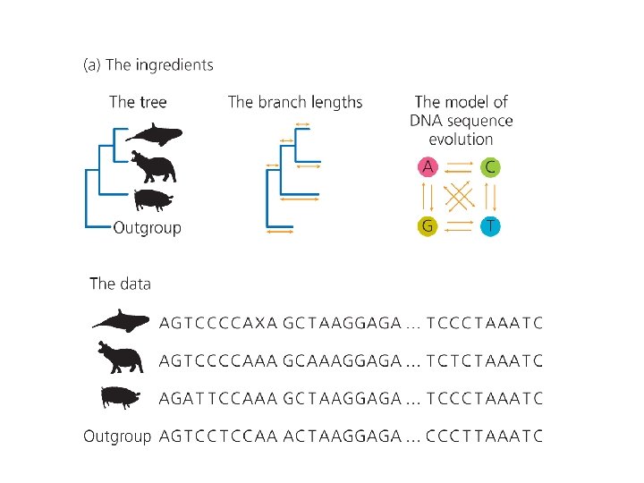
Patterns in Evolution I. Phylogenetic A. Systematics: Taxonomy and Classification B. Reconstructing Phylogenies 1. Characters 2. Trees 3. Molecular Evolution and Algorithms DNA, RNA, and protein sequence data: - thousands of characters - multiple parsimonious trees

3. Molecular Evolution and Algorithms a. Synapomorphies and parsimony Are cetaceans artiodactyls, or a sister group to the Artiodactyla?

3. Molecular Evolution and Algorithms a. Synapomorphies and parsimony Exon 7 from the gene that encodes β-casein, a protein in milk. Shared derived traits with cetaceans at positions 162, 166, 177

3. Molecular Evolution and Algorithms a. Synapomorphies and parsimony 6 changes required at these positions; 41 over entire 60 base sequence 9 changes required at these positions; 47 over entire 60 base sequence

3. Molecular Evolution and Algorithms a. Synapomorphies and parsimony 6 changes required at these positions; 41 over entire 60 base sequence 9 changes required at these positions; 47 over entire 60 base sequence

PROBLEMS WITH BASE DATA • Scoring characters-its easy if its categorical (A, C, T, G), but very difficult if it is continuous. Need independent characters, so they are weighted evenly. • Homoplasies are common - both as convergence or reversal. • Ancient changes are obscured by more recent ones. . . A to G, then G to C, looks like it could be one change A to C. • Rapid radiations mean that branches/subgroups may not have had time to evolve their own unique synapomorphies. . . and we have lots of species with autapomorphies (and are thus distinct) but it is difficult to group them. • Trees of single genes may not "map" onto the phylogenetic tree among species. The loss of particular alleles may not parallel patterns of relationships. • Hybridization and gene transfer - this can make populations look more similar at these loci than they really are across the whole genome. • Rates of evolution of different characters and states differ. . . Some are "highly conserved' and don't change much. . . others change dramatically. This is called mosaic evolution. This affects the "branch lengths" that are used to represent the degree of departure (or the quantified number of genetic changes in that unique lineage.

Patterns in Evolution I. Phylogenetic A. Systematics: Taxonomy and Classification B. Reconstructing Phylogenies 1. Characters 2. Trees 3. Molecular Evolution and Algorithms DNA, RNA, and protein sequence data: - thousands of characters - multiple parsimonious trees a. Synapomorphies and parsimony b. UPGMA (unweighted pair group method with arithmetic mean)

3. Molecular Evolution and Algorithms b. UPGMA - UPGMA assume constant mutation rates, and so is the simplest likelihood model. Unweighted Pair Group Method with Arithmetic Mean These are the number of differences in AA sequences between species-pairs.

3. Molecular Evolution and Algorithms b. UPGMA • The most similar sequences are those of humans and monkey (1 difference). • This difference accumulated over TWO lineages since their divergence (constant mutation) • So, the branch length of each is 1 difference / 2 branches = 0. 5

1. So, we join taxa B (human) and F (monkey). 2. Then, we AVERAGE the differences between these taxa and each other taxon and reduce the matrix. . so, B differs from A by 19 AA's, and F differs from A by 18 AA's. So the average difference between A and new taxon 'BF' = 18. 5 (fusion of two orange boxes into one orange box in the new and reduced matrix). (That's why this is called UPGMA - unweighted pair -group method using arithmetic averages)

1. So, we join taxa B (human) and F (monkey). 2. Then, we AVERAGE the differences between these taxa and each other taxon and reduce the matrix. . so, B differs from A by 19 AA's, and F differs from A by 18 AA's. So the average difference between A and new taxon 'BF' = 18. 5 (fusion of two orange boxes into one orange box in the new and reduced matrix). 3. Now, in the reduced matrix, we look for the most similar pair (which is A and D = 8 diffs). We halve the difference to calculate each unique branch length (4. 0)

1. So, we join taxa B (human) and F (monkey). 2. Then, we AVERAGE the differences between these taxa and each other taxon and reduce the matrix. . so, B differs from A by 19 AA's, and F differs from A by 18 AA's. So the average difference between A and new taxon 'BF' = 18. 5 (fusion of two orange boxes into one orange box in the new and reduced matrix). 3. Now, in the reduced matrix, we look for the most similar pair (which is A and D = 8 diffs). We halve the difference to calculate each unique branch length (4. 0) 4. Now repeat the averaging process with other taxa to reduce the matrix.

3. Molecular Evolution and Algorithms b. UPGMA Here, branch lengths are equal (and additive) because averaging and constant mutation are assumed. In other models, branch lengths vary – reflecting more complex models which accept different substitution rates.

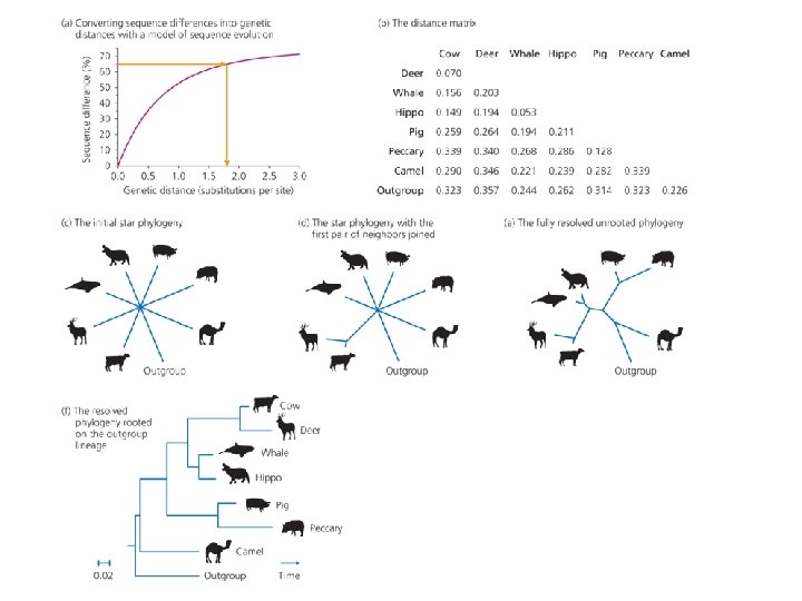
3. Molecular Evolution and Algorithms a. Synapomorphies and parsimony b. UPGMA c. Branch Length Units 1) In the UPGMA example, the Branch length is “mean number of AA substitutions” in cytochrome C. This protein has 104 AA in animals. 2) Typically, these raw data are Converted to “nucleotide substitutions per site” by dividing #/length. Or, by Multiplying this by 100, as % change. 18 differences. 18/104 AA = 0. 173 nucleotide substitutions per site 0. 17 x 100 = 17. 3 % difference

3. Molecular Evolution and Algorithms a. Synapomorphies and parsimony b. UPGMA c. Branch Length Units 1) In the UPGMA example, the Branch length is “mean number of AA substitutions” in cytochrome C. This protein has 104 AA in animals. 2) Typically, these raw data are Converted to “nucleotide substitutions per site” by dividing #/length. Or, by Multiplying this by 100, as % change. 18 differences. 18/104 AA = 0. 173 nucleotide substitutions per site 0. 17 x 100 = 17. 3 % difference 3) If AA have been sequenced, data is often transformed to “minimum nucleotide substitutions” using the genetic code. Changing LEU to PRO requires at least 1 nucleotide substitution, but LEU to THR requires at least 2 substitutions.

3. Molecular Evolution and Algorithms a. Synapomorphies and parsimony b. UPGMA c. Branch Length Units 4) Evolutionary Modeling The relationship between % difference and evolutionary divergence (substitution rate) may not be linear. - not all differences are indicative of change; Even 2 random sequences will only differ by 75% (just by chance there will be the same base at 25% of sites). - some changes are more likely than others. Transition mutations (A to G, C to T) are more likely than transversions (A to C or T). So, models incorporate a “transition/transversion ratio” (2. 0, above right).

3. Molecular Evolution and Algorithms a. Synapomorphies and parsimony b. UPGMA c. Branch Length Units 4) Evolutionary Modeling The relationship between % difference and evolutionary divergence (substitution rate) May not be linear. - Our ability to detect change depends on existing degree of similarity. We are more likely to detect changes in sequences that are identical, than in sequences that are only 50% similar, because many changes in that case will make the sequences MORE SIMILAR. So a change in similarity from 10 -12% probably represents fewer mutations, and less “genetic distance”, than observed changes from 60 -62%. If sequences are 60% different, a lot of mutations in one sequence will make it more similar to the other…thus the same NET change of 2% represents MORE evolutionary change (Distance).

3. Molecular Evolution and Algorithms a. Synapomorphies and parsimony b. UPGMA c. Branch Length Units d. Calculating Branch Lengths A A B B C 22 39 41 C D E Hypothetical % sequence differences A B a c C b 1) a + b = 22 2) a + c = 39 3) b + c = 41 4) = 2 – 3 = a – b = -2 5) = 1 + 4 = 2 a = 20, so a = 10. 6) The distance from A to B = 22, so b = 12, and C = 29. OR a = ((AC – BC) + AB) / 2

3. Molecular Evolution and Algorithms a. Synapomorphies and parsimony b. UPGMA c. Branch Length Units d. Calculating Branch Lengths A A B C D E 22 39 39 41 41 41 43 18 20 10 E Hypothetical % sequence differences among 5 taxa

3. Molecular Evolution and Algorithms a. Synapomorphies and parsimony b. UPGMA c. Branch Length Units d. Calculating Branch Lengths A A B C D E 22 39 39 41 41 41 43 18 20 10 E Hypothetical % sequence differences among 5 taxa 1) D and E are most similar 2) Calculate average distance from D and E to A, B, and C (reduce this to a 3 -point problem)

3. Molecular Evolution and Algorithms a. Synapomorphies and parsimony b. UPGMA c. Branch Length Units d. Calculating Branch Lengths A A B C D E 22 39 39 41 41 41 43 18 20 10 E Hypothetical % sequence differences among 5 taxa 1) D and E are most similar 2) Calculate average distance from D and E to A, B, and C (D = 32. 6, E = 34. 6) 3) So, E is 2 units farther away from node, and the distance between them is 10, so:

D a D and E are the closest sequences A-C D E - 32. 6 34. 6 - 10 D E A-C c b a=4 b=6 E a = ((AC – BC) + AB) / 2 - Now let’s recompute the complete distance matrix A A B C D E 22 39 39 41 41 41 43 18 20 10 A B C DE - 22 39 40 - 41 42 - 19 - C and DE are the closet sequences

D a D and E are the closest sequences A-C D E - 32. 6 34. 6 - 10 D E A-C c b a=4 b=6 E a = ((AC – BC) + AB) / 2 - Now let’s recompute the complete distance matrix A A B C D E 22 39 39 41 41 41 43 18 20 10 E Mean distance from C to AB = 40, and mean distance from DE to AB = 41. A B C DE - 22 39 40 - 41 42 - 19 - C and DE are the closet sequences

C and DE are the closet sequences AB AB C - C DE 40 41 - 19 DE C a b is not just for that segment, it represents the complete distance from the connecting node to the leaves c A-B b a=9 b = 10 (mean) - So once again, there is one unit of branch length difference to the node of C and DE, with a total distance of 19. DE a = ((AC – BC) + AB) / 2 9 Now let’s recompute the complate distance matrix A B C DE - 22 39 40 - C 31 A-B 5 41 42 - 19 B - E A A B CDE - 22 39. 5 - 41. 5 - 4 D 6 E

A Now we are in thee trivial case of 3 sequences A A B C-E - 22 39. 5 - 41. 5 B C-E a b B c CDE a = 10 b = 12 - b is not just for that segment, it represents the complete distance from the connecting node to the leaves a = ((AC – BC) + AB) / 2 A C 9 10 20 5 B 4 12 D 6 E

10 WHICH was the outgroup? 20 12 Lets Say C 6 E 5 4 D 9 A C 9 10 C 20 5 B 4 12 D 6 E A B

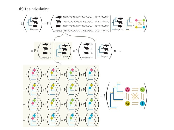
3. Molecular Evolution and Algorithms a. Synapomorphies and parsimony b. UPGMA c. Branch Length Units d. Calculating Branch Lengths e. Maximum Likelihood Models What evolutionary rates (in terms of transitions and tranversion, etc. , are required to give us the pattern and rate (as measured in branch lengths) that we SEE? So, different models of evolution are tested. The models are probability matrices of substitution rates between bases. A tree is given. The branch lengths are given. The model of mutation changes, and the probabilities of generating the data (sequences) change with the model. The “likelihood” of a tree is the probability that it generates the data.

3. Molecular Evolution and Algorithms a. Synapomorphies and parsimony b. UPGMA c. Branch Length Units d. Calculating Branch Lengths e. Maximum Likelihood Models f. Neighbor Joining Similar, but we don’t prioritize which pair we group first. Rather, we repeat the tree formation using every possible pair-wise combination, and then pick the tree with the shortest total branch lengths (most conservative evolutionary tree). Repeat, using this pair as one node (like “DE” before).

3. Molecular Evolution and Algorithms a. Synapomorphies and parsimony b. UPGMA c. Branch Length Units d. Calculating Branch Lengths e. Maximum Likelihood Models f. Neighbor Joining g. Bootstrapping Gain confidence in a node by subsampling the data and creating a tree. Is the node still there? How frequently is it present in 100 or 1000 subsamples of the data set?

Randomly sample characters (in this case, base positions) WITH REPLACEMENT. Create the tree, and report the frequency of a clade in the tree.

Bootstrap using entire 1100 bases of casein gene, N = 1000. Whales are within the Artiodactyla in 99% of clades. Whales are in clade with deer, hippo, cow (100%)

3. Molecular Evolution and Algorithms a. Synapomorphies and parsimony b. UPGMA c. Branch Length Units d. Calculating Branch Lengths e. Maximum Likelihood Models f. Neighbor Joining g. Bootstrapping h. Bayesian inference

1) Must estimate the prior probability of trees… based on external knowledge. Or, assume equality. Likelihood pp P(tree|data) = P(data|tree) P(data) Where P(data) = SUM(tree likelihood x prior prob) across all trees considered. So, for the trees considered and given their prior probabilities, what is their fractional probability at which the data produces each tree? This is the posterior probability that we want…. P(tree|data).

1) Must estimate the prior probability of trees… based on external knowledge. Or, assume equality. Likelihood pp P(tree|data) = P(data|tree) P(data) Where P(data) = SUM(tree likelihood x prior prob) across all trees considered. So, for the trees considered and given their prior probabilities, what is their fractional probability at which the data produces each tree? This is the posterior probability. Clade credibility is the sum of the probabilities of the trees in which it occurs.

3. Molecular Evolution and Algorithms a. Synapomorphies and parsimony b. UPGMA c. Branch Length Units d. Calculating Branch Lengths e. Maximum Likelihood Models f. Neighbor Joining g. Bootstrapping h. Baysian inference i. SINE’s and LINE’s - Short and Long interspersed sequences – transposable elements. - Highly unlikely to end up in the same place in the genome by chance… - Similarity is most likely a SHARED, DERIVED character.