Parkes The Dish M 83 19 Parkes The

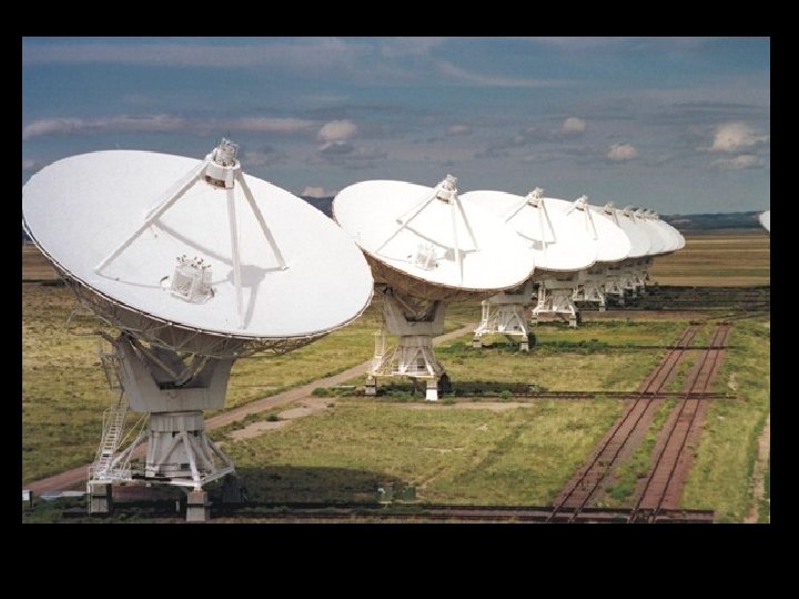
Parkes “The Dish”

M 83 19’

Parkes “The Dish”

VLA, Very Large Array New Mexico

Arecibo Telescope… in Puerto Rico 300 metres

GBT Green Bank West Virginia … the newest… … and last (perhaps)… … big dish Unblocked Aperture 91 metres

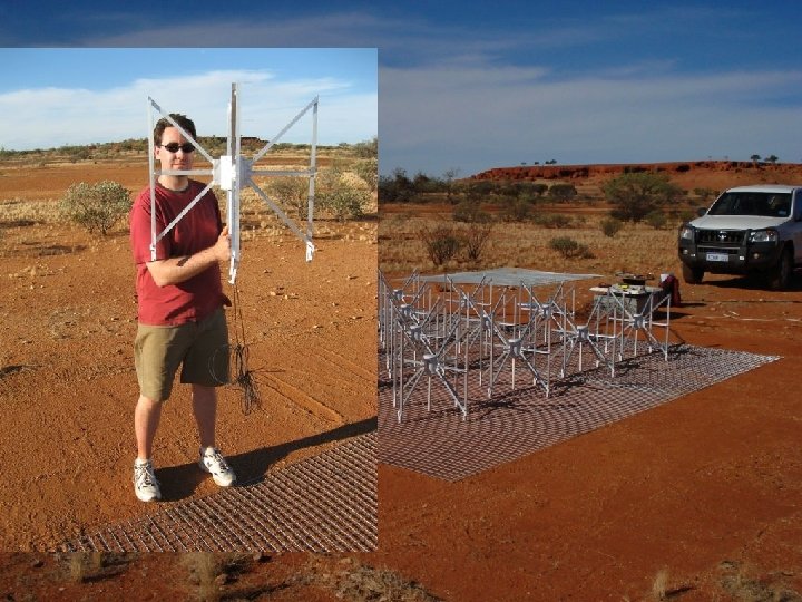
LOFAR “elements”

http: //www. astron. nl/press/250407. htm

LOFAR image at ~ 50 MHz (Feb 2007)

Dipole + ground plane: plane a model conducting ground plane

Dipole + ground plane Ioe i 2 pft equivalent to dipole plus mirror image -Ioe i 2 pft

4 x 4 array of dipoles on ground plane - the ‘LFD’ element h s s (many analogies to gratings for optical wavelengths)

4 x 4 Tuned for 150 MHz sin projection Beam Reception Pattern

‘sin projection’ gives little weight to sky close to horizon !

As function of angle away from Zenith ZA = 0 deg 45 15 60 30 75

q = zenith angle Ioe i 2 pft h h equivalent to dipole plus mirror image -Ioe i 2 pft 2 P(q) ~ sin [2 ph cos(q)/l] (maximize response at q=0 if h=l/4 )

As function of frequency 4 x 4 Patterns • • ZA = 30 deg tuned for 150 MHz 120 150 180 210 240

Very Large Array USA Atacama L Millimeter Array Westerbork Telescope Netherlands

VLBA Very Long Baseline Array for: Very Long Baseline Interferometry

EVN: European VLBI Network (more and bigger dishes than VLBA) LBA: Long Baseline Array in AU

ESO Paranal, Chile

* *** (biblical status in field)

More references: • Synthesis Imaging in Radio Astronomy, 1998, ASP Conf. Series, Vol 180, eds. Taylor, Carilli & Perley • Single-Dish Radio Astronomy, 2002, ASP Conf. Series, Vol 278, eds. Stanimirovic, Altschuler, Goldsmith & Salter • AIPS Cookbook, http: //www. aoc. nrao. edu/aips/

LOFAR + MWA ATCA GMRT VLA ALMA 350 m 10 MHz ground based radio techniques

Radio “Sources” Spectra: 1) Thermal 2) Non-Thermal 1) Thermal Flux Density emission mechanism related to Planck BB… electrons have ~Maxwellian distribution 2) Non-Thermal emission typically from relativistic electrons in magnetic field… electrons have ~power law energy distribution Distinctive Radio Spectra ! Frequency MHz

Nonthermal

M 81 Group of Galaxies Visible Light Thermal Radio map of cold hydrogen gas

(from P. Mc. Gregor notes)

In where In ~ Sn/W can assign “brightness temperature” to objects where “Temp” really has no meaning…

Flux Density [Jansky] Brightest Sources in Sky Frequency MHz (from Kraus, Radio Astronomy)

Radio `source’ Goals of telescope: • maximize collection of energy (sensitivity or gain) • isolate source emission from other sources… (directional gain… dynamic range) Collecting area

Radio telescopes are Diffraction Limited Incident waves

Radio telescopes are Diffraction Limited q Waves arriving from slightly different direction have Incident waves Phase gradient across aperture… When get cancellation: Resolution = q ~ l/D l/2,

Celestial Radio Waves?

Actually……. Noise …. time series Time Fourier transform Frequency

F. T. of noise time series Frequency Narrow band filter B Hz Frequency Envelope of time series varies on scale t ~ 1/B sec Time

Observe “Noise” …. time series V(t) Time Fourier transform Frequency

…want “Noise Power” … from voltage time series => V(t)2 then average power samples V(t) “integration” Time Fourier transform Frequency

Radio sky in 408 MHz continuum (Haslam et al)

Difference between pointing at Galactic Center and Galactic South Pole at the LFD in Western Australia Power ~4 MHz band Frequency

thought experiment… Cartoon antenna 2 wires out (antennas are “reciprocal” devices… can receive or broadcast)

thought experiment… Black Body oven at temperature = T

thought experiment… R Black Body oven at temperature = T

thought experiment… … wait a while… reach equilibrium… at T R Black Body oven at temperature = T warm resistor delivers power P = k. T B (B = frequency bandwidth; k = Boltzmann Const)

real definition… Measure Antenna output Power as “Ta” = antenna temperature Ta R temp = T warm resistor produces P = k. T B = Pa = k. Ta B

Radio `source’ Q Reception Pattern or Power Pattern “Sidelobes” Collecting area

Radio `source’ If source with brightness temperature Tb fills the beam (reception pattern), then Ta = Tb Collecting area (!! No dependence on telescope if emission fills beam !!)

receiver “temperature”… quantify Receiver internal noise Power as “Tr” = “receiver temperature” Ta Ampl, etc Real electronics adds noise …treat as ideal, noise-free amp with added power from warm R Ampl, etc Tr+Ta

“system temperature”… quantify total receiver System noise power as “Tsys” [include spillover, scattering, etc] Tsys+Ta Ampl, etc RMS fluctuations = DT DT = (fac)Tsys/(B tint)1/2 Fac ~ 1 – 2 B = Bandwidth, Hz tint = integration time, seconds

Radio `point source’ Power collected = Sn Aeff B/2 Sn = flux density (watts/sq-m/Hz) [ 1 Jansky = 1 Jy = 10 -26 w/sq-m/Hz ] Aeff = effective area (sq-m) B = frequency bandwith (Hz) Ta = Sn Aeff /2 k Collecting area

“Resolved” If source fills the beam Ta = T b “Unresolved” Sn = flux density Aeff = effective area Ta = Sn Aeff /2 k RMS = DT = (fac)Tsys/(B tint)1/2 (sq-m) fac ~ 1 – 2 B = Bandwidth tint = integration time

Example 1 High Velocity HI Cloud: NHI = 1 x 1019 cm-2 NHI = 1. 8 x 1018 Tb DV km/s = 1. 8 x 1018 Tb (10) Tb = 0. 6 K B = (10/3 x 105)x 1420 x 106 = 50 KHz 5 rms = 5 DT = Tb = 0. 6 K rms = DT = (fac)Tsys/(B tint)1/2 = (1)(30)/(B tint)1/2 tint = (30/0. 12)2/(50 x 103) = 1. 2 seconds (To reach NHI = 1 x 1017 cm-2 need 10, 000 times longer ~ 3 hours)

Example 2 High redshift quasar with continuum flux density Sn = 100 m. Jy (Ta = Sn Aeff /2 k) Ka = Ta / Sn = Aeff /2 k [K/Jy] = 0. 7 K/Jy Parkes = 10 K/Jy Arecibo = 2. 7 K/Jy VLA = 300 K/Jy SKA Parkes: 100 m. Jy yields Ta = 70 m. K 64 MHz continuum bandwidth for receiver 5 rms = 5 DT = Tb = 0. 07 K rms = DT = (fac)Tsys/(B tint)1/2 = (1)(30)/(B tint)1/2 tint = (30/0. 014)2/(64 x 106) ~ 0. 1 sec

Example 3: Array High redshift quasar with continuum flux density Sn = 1 m. Jy (Ta = Sn Aeff /2 k) Ka = Ta / Sn = Aeff /2 k [K/Jy] = 0. 7 K/Jy Parkes = 6 x 0. 1 = 0. 6 K/Jy ACTA rms = DS = (fac)(Tsys /Ka)/(B tint)1/2 ATCA (B=128 MHz): 1 m. Jy = 5 rms means DS = 0. 2 m. Jy rms = DS = (fac)(Tsys /Ka)/(B tint)1/2 = (1. 4)(30/0. 6)/(B tint)1/2 tint = (70/0. 0002)2/(128 x 106) ~ 16 min