On Applications of Rough Sets theory to Knowledge

On Applications of Rough Sets theory to Knowledge Discovery Frida Coaquira UNIVERSITY OF PUERTO RICO MAYAGÜEZ CAMPUS frida_cn@math. uprm. edu

Introduction One goal of the Knowledge Discovery is extract meaningful knowledge. Rough Sets theory was introduced by Z. Pawlak (1982) as a mathematical tool for data analysis. Rough sets have many applications in the field of Knowledge Discovery: feature selection, discretization process, data imputations and create decision Rules. Rough set have been introduced as a tool to deal with, uncertain Knowledge in Artificial Intelligence Application.

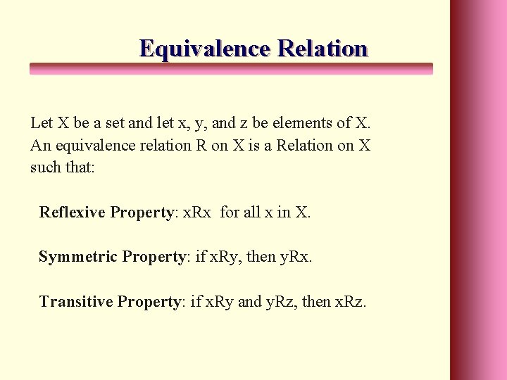
Equivalence Relation Let X be a set and let x, y, and z be elements of X. An equivalence relation R on X is a Relation on X such that: Reflexive Property: x. Rx for all x in X. Symmetric Property: if x. Ry, then y. Rx. Transitive Property: if x. Ry and y. Rz, then x. Rz.

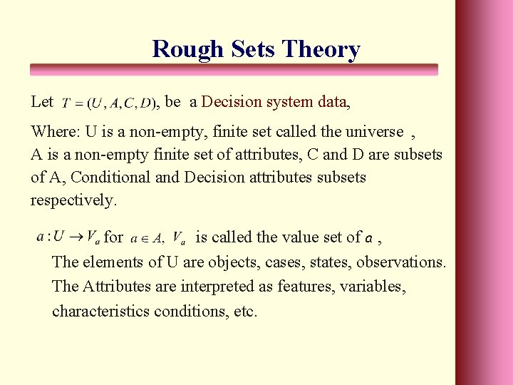
Rough Sets Theory Let , be a Decision system data, Where: U is a non-empty, finite set called the universe , A is a non-empty finite set of attributes, C and D are subsets of A, Conditional and Decision attributes subsets respectively. for is called the value set of a , The elements of U are objects, cases, states, observations. The Attributes are interpreted as features, variables, characteristics conditions, etc.

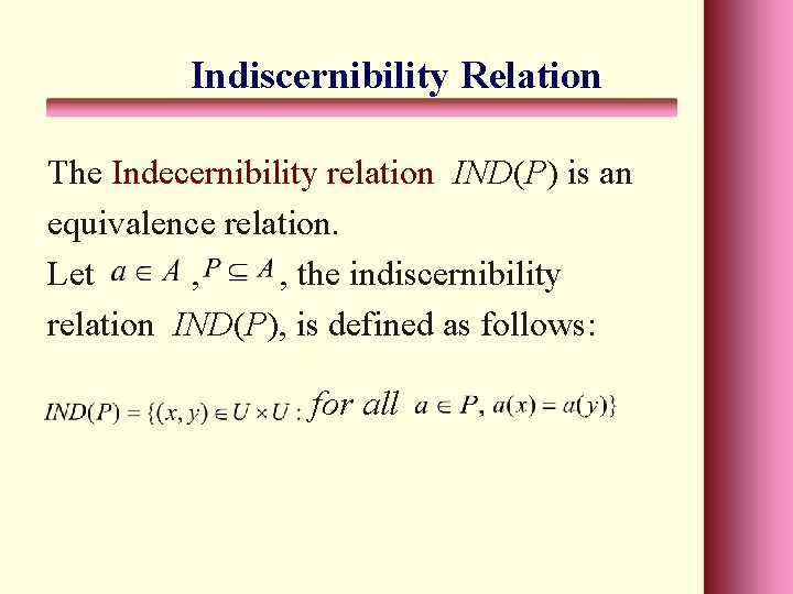
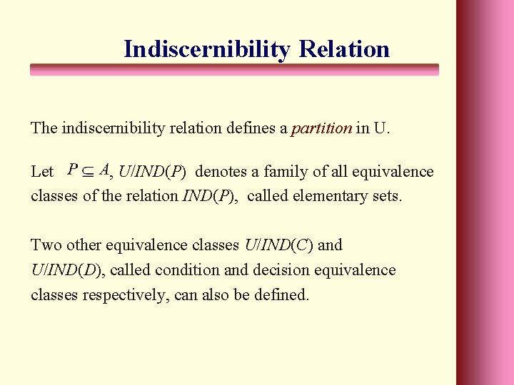
Indiscernibility Relation The Indecernibility relation IND(P) is an equivalence relation. Let , , the indiscernibility relation IND(P), is defined as follows: for all

Indiscernibility Relation The indiscernibility relation defines a partition in U. Let , U/IND(P) denotes a family of all equivalence classes of the relation IND(P), called elementary sets. Two other equivalence classes U/IND(C) and U/IND(D), called condition and decision equivalence classes respectively, can also be defined.

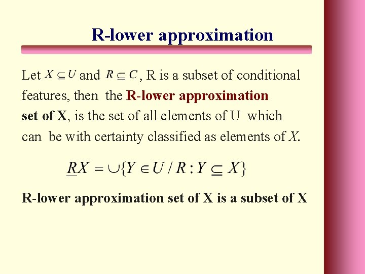
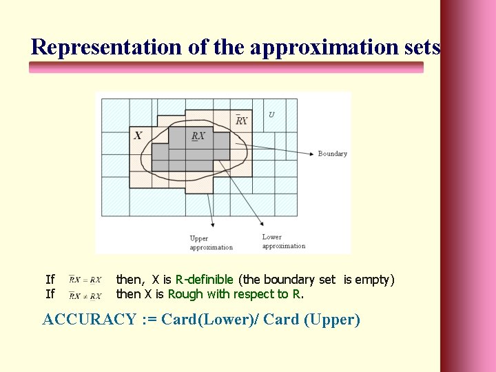
R-lower approximation Let and , R is a subset of conditional features, then the R-lower approximation set of X, is the set of all elements of U which can be with certainty classified as elements of X. R-lower approximation set of X is a subset of X

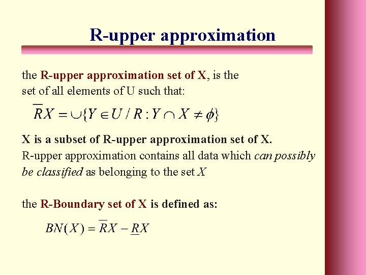
R-upper approximation the R-upper approximation set of X, is the set of all elements of U such that: X is a subset of R-upper approximation set of X. R-upper approximation contains all data which can possibly be classified as belonging to the set X the R-Boundary set of X is defined as:

Representation of the approximation sets If If then, X is R-definible (the boundary set is empty) then X is Rough with respect to R. ACCURACY : = Card(Lower)/ Card (Upper)

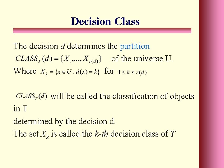
Decision Class The decision d determines the partition of the universe U. Where for will be called the classification of objects in T determined by the decision d. The set Xk is called the k-th decision class of T

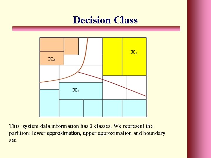
Decision Class This system data information has 3 classes, We represent the partition: lower approximation, upper approximation and boundary set.

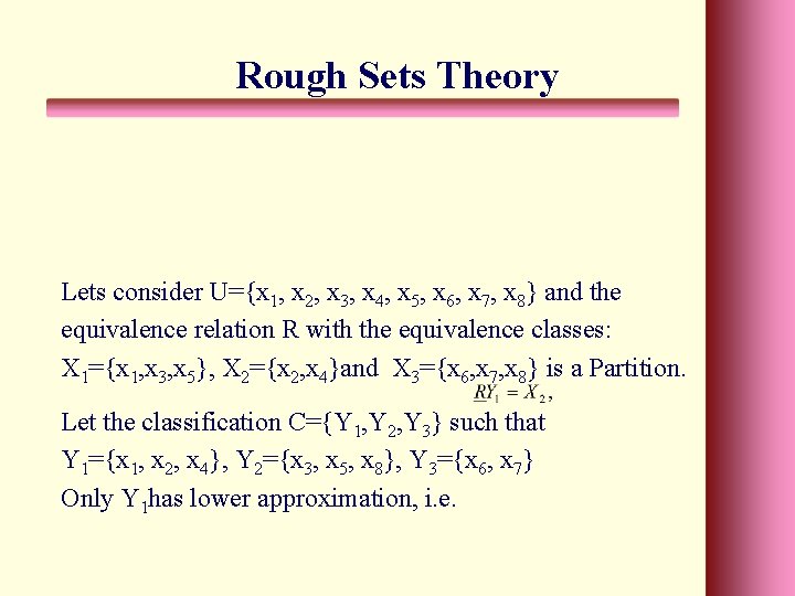
Rough Sets Theory Lets consider U={x 1, x 2, x 3, x 4, x 5, x 6, x 7, x 8} and the equivalence relation R with the equivalence classes: X 1={x 1, x 3, x 5}, X 2={x 2, x 4}and X 3={x 6, x 7, x 8} is a Partition. Let the classification C={Y 1, Y 2, Y 3} such that Y 1={x 1, x 2, x 4}, Y 2={x 3, x 5, x 8}, Y 3={x 6, x 7} Only Y 1 has lower approximation, i. e.

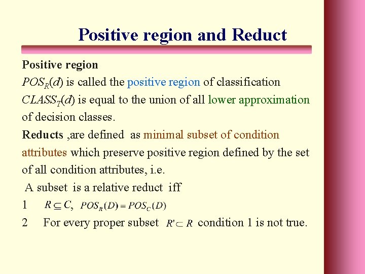
Positive region and Reduct Positive region POSR(d) is called the positive region of classification CLASST(d) is equal to the union of all lower approximation of decision classes. Reducts , are defined as minimal subset of condition attributes which preserve positive region defined by the set of all condition attributes, i. e. A subset is a relative reduct iff 1 , 2 For every proper subset condition 1 is not true.

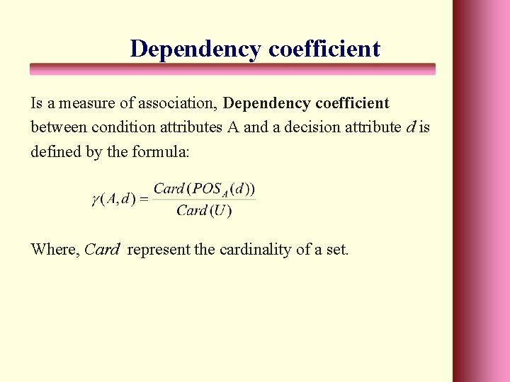
Dependency coefficient Is a measure of association, Dependency coefficient between condition attributes A and a decision attribute d is defined by the formula: Where, Card represent the cardinality of a set.

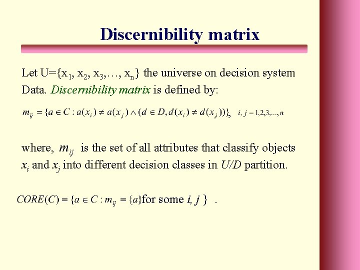
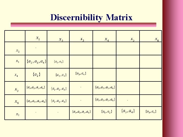
Discernibility matrix Let U={x 1, x 2, x 3, …, xn} the universe on decision system Data. Discernibility matrix is defined by: , where, is the set of all attributes that classify objects xi and xj into different decision classes in U/D partition. for some i, j }.

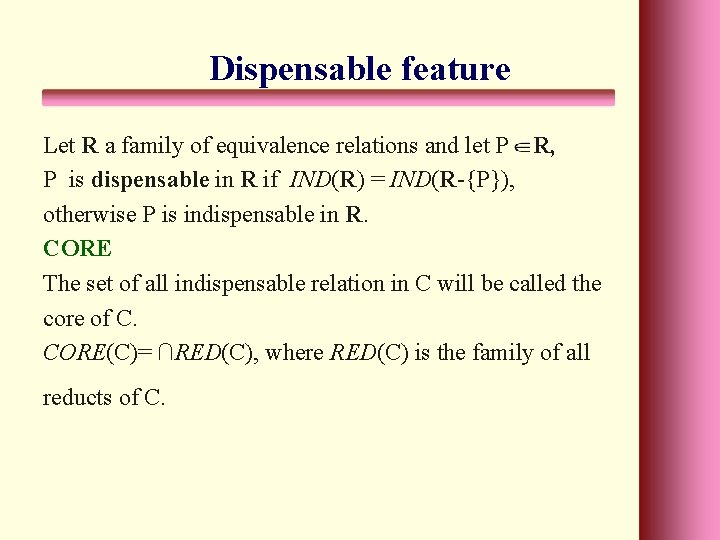
Dispensable feature Let R a family of equivalence relations and let P R, P is dispensable in R if IND(R) = IND(R-{P}), otherwise P is indispensable in R. CORE The set of all indispensable relation in C will be called the core of C. CORE(C)= ∩RED(C), where RED(C) is the family of all reducts of C.

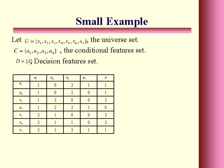
Small Example , Let{, , , the universe set. , the conditional features set. , Decision features set. {, {, d 1 0 2 1 1 1 0 2 0 1 1 2 0 0 2 1 2 2 1 0 0 2 2 1 1

Discernibility Matrix - - -

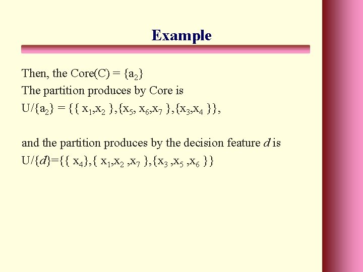
Example Then, the Core(C) = {a 2} The partition produces by Core is U/{a 2} = {{ x 1, x 2 }, {x 5, x 6, x 7 }, {x 3, x 4 }}, and the partition produces by the decision feature d is U/{d}={{ x 4}, { x 1, x 2 , x 7 }, {x 3 , x 5 , x 6 }}

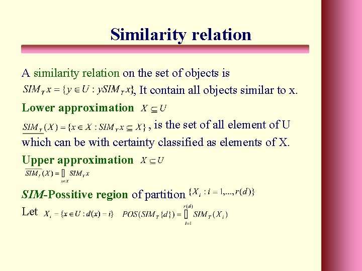
Similarity relation A similarity relation on the set of objects is , It contain all objects similar to x. Lower approximation , is the set of all element of U which can be with certainty classified as elements of X. Upper approximation SIM-Possitive region of partition Let

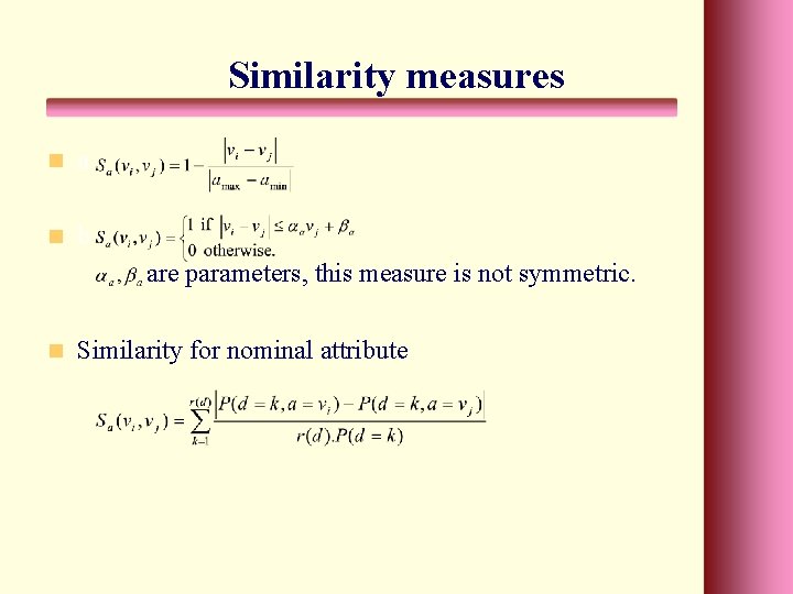
Similarity measures n a n b are parameters, this measure is not symmetric. n Similarity for nominal attribute

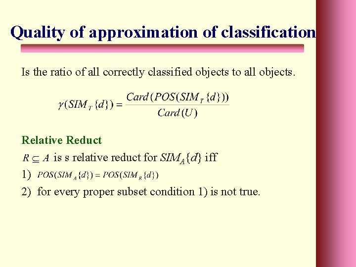
Quality of approximation of classification Is the ratio of all correctly classified objects to all objects. Relative Reduct is s relative reduct for SIMA{d} iff 1) 2) for every proper subset condition 1) is not true.

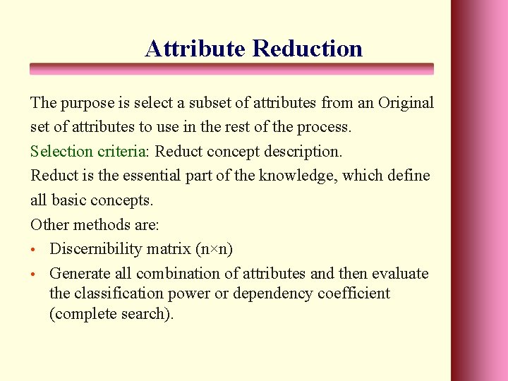
Attribute Reduction The purpose is select a subset of attributes from an Original set of attributes to use in the rest of the process. Selection criteria: Reduct concept description. Reduct is the essential part of the knowledge, which define all basic concepts. Other methods are: • Discernibility matrix (n×n) • Generate all combination of attributes and then evaluate the classification power or dependency coefficient (complete search).

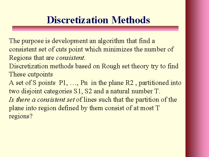
Discretization Methods The purpose is development an algorithm that find a consistent set of cuts point which minimizes the number of Regions that are consistent. Discretization methods based on Rough set theory to find These cutpoints A set of S points P 1, …, Pn in the plane R 2 , partitioned into two disjoint categories S 1, S 2 and a natural number T. Is there a consistent set of lines such that the partition of the plane into region defined by them consist of at most T regions?

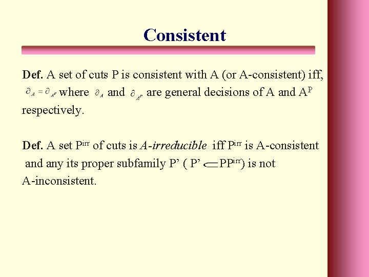
Consistent Def. A set of cuts P is consistent with A (or A-consistent) iff, where and are general decisions of A and AP respectively. Def. A set Pirr of cuts is A-irreducible iff Pirr is A-consistent and any its proper subfamily P’ ( P’ PPirr) is not A-inconsistent.

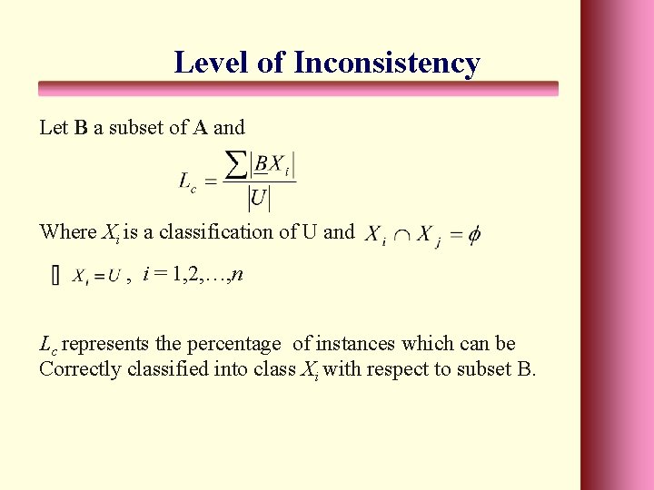
Level of Inconsistency Let B a subset of A and Where Xi is a classification of U and , i = 1, 2, …, n Lc represents the percentage of instances which can be Correctly classified into class Xi with respect to subset B.

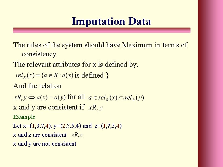
Imputation Data The rules of the system should have Maximum in terms of consistency. The relevant attributes for x is defined by. is defined } And the relation for all x and y are consistent if. Example Let x=(1, 3, ? , 4), y=(2, ? , 5, 4) and z=(1, ? , 5, 4) x and z are consistent x and y are not consistent

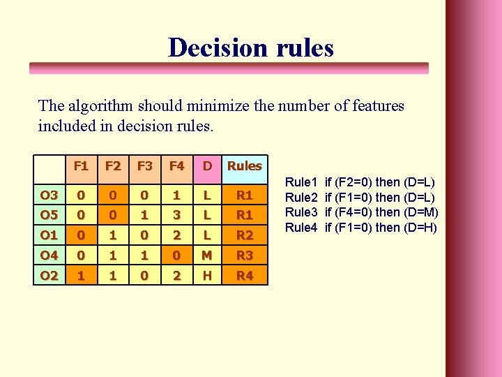
Decision rules The algorithm should minimize the number of features included in decision rules. F 1 F 2 F 3 F 4 D Rules O 3 0 0 0 1 L R 1 O 5 0 0 1 3 L R 1 O 1 0 2 L R 2 O 4 0 1 1 0 M R 3 O 2 1 1 0 2 H R 4 Rule 1 Rule 2 Rule 3 Rule 4 if (F 2=0) then (D=L) if (F 1=0) then (D=L) if (F 4=0) then (D=M) if (F 1=0) then (D=H)

References [1] Gediga, G. And Duntsch, I. (2002) Maximum Consistency of Incomplete Data Via Non-invasive Imputation. Artificial Intelligence. [2] Grzymala, J. and Siddhave, S. (2004) Rough set Approach to Rule Induction from Incomplete Data. Proceeding of the IPMU’ 2004, the 10 th International Conference on information Processing and Management of Uncertainty in Knowledge-Based System. [3] Pawlak, Z. (1995) Rough sets. Proccedings of the 1995 ACM 23 rd annual conference on computer science. [4]Tay, F. and Shen, L. (2002) A modified Chi 2 Algorithm for Discretization. In IEEE Transaction on Knowledge and Data engineering, Vol 14, No. 3 may/june. [5] Zhong, N. (2001) Using Rough Sets with Heuristics for Feature Selection. Journal of Intelligent Information Systems, 16, 199 -214, Kluwer Academic Publishers.

THANK YOU!