NRCSE Statistics data and deterministic models Some issues

NRCSE Statistics, data, and deterministic models

Some issues in model assessment Spatiotemporal misalignment Grid boxes vs observations Types of error Measurement error and bias Model error Approximation error Manipulate data or model output? Two case studies: SARMAP – kriging MODELS-3 – Bayesian melding Other uses of Bayesian hierarchical models

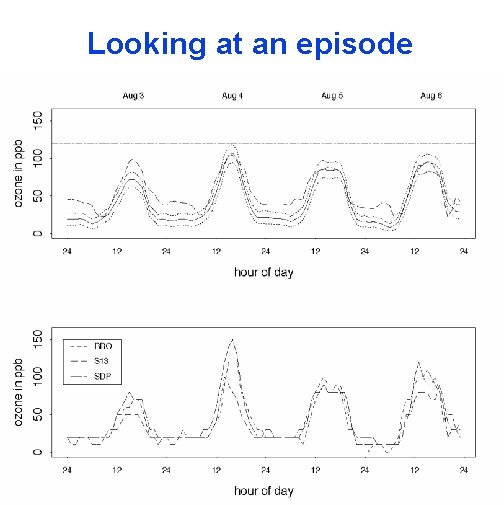
Assessing the SARMAP model 60 days of hourly observations at 32 sites in Sacramento region Hourly model runs for three “episodes”

Task Estimate from data the ozone level at x’s in a grid square. Use sum to estimate integral over grid square. Issues: Transformation Diurnal cycle Temporal dependence Spatial dependence Space-time interaction

Transformation Heterogeneous variability–mean and variance positively related Square root transformation All modeling now on square root scale– approximately normal

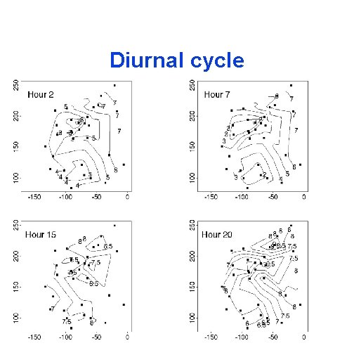
Diurnal cycle

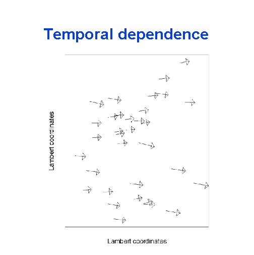
Temporal dependence

Spatial dependence

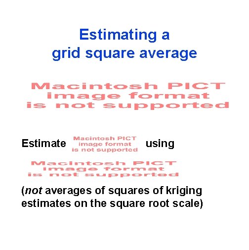
Estimating a grid square average Estimate using (not averages of squares of kriging estimates on the square root scale)

Looking at an episode

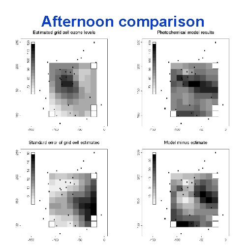
Afternoon comparison

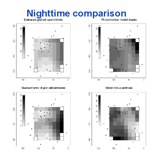
Nighttime comparison

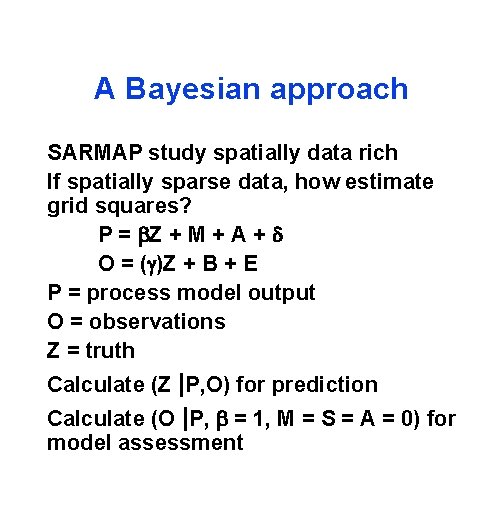
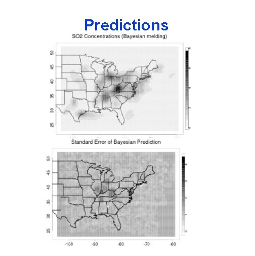
A Bayesian approach SARMAP study spatially data rich If spatially sparse data, how estimate grid squares? P = Z + M + A + O = ( )Z + B + E P = process model output O = observations Z = truth Calculate (Z |P, O) for prediction Calculate (O |P, = 1, M = S = A = 0) for model assessment

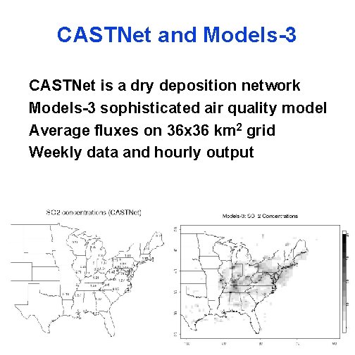
CASTNet and Models-3 CASTNet is a dry deposition network Models-3 sophisticated air quality model Average fluxes on 36 x 36 km 2 grid Weekly data and hourly output

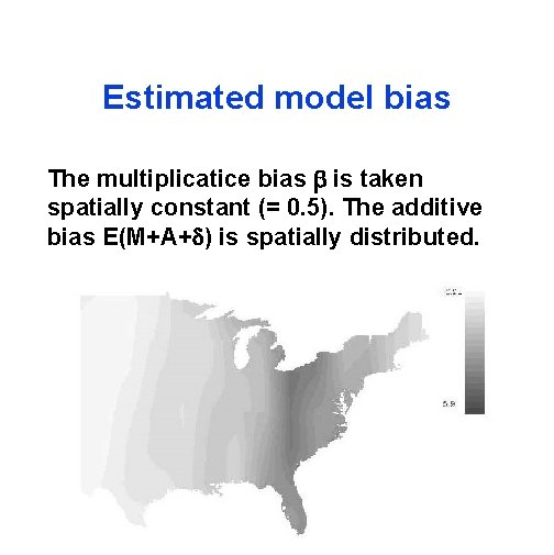
Estimated model bias The multiplicatice bias is taken spatially constant (= 0. 5). The additive bias E(M+A+ ) is spatially distributed.

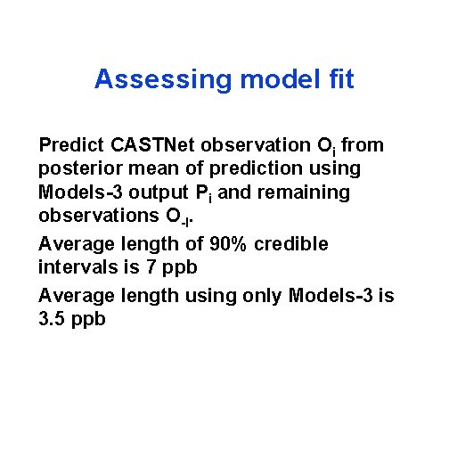
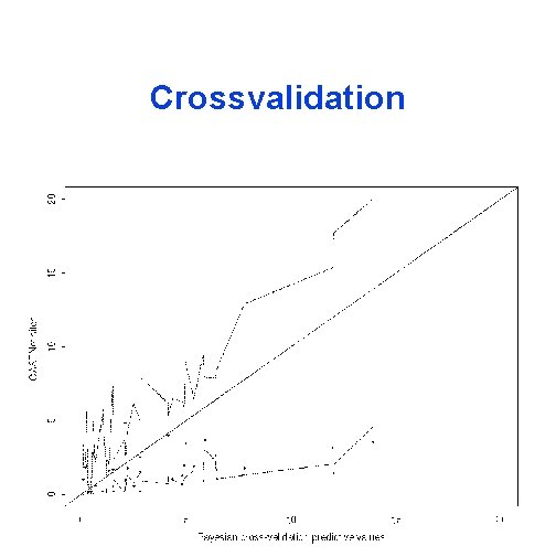
Assessing model fit Predict CASTNet observation Oi from posterior mean of prediction using Models-3 output Pi and remaining observations O-I. Average length of 90% credible intervals is 7 ppb Average length using only Models-3 is 3. 5 ppb

Crossvalidation

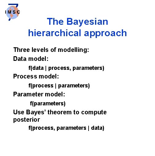
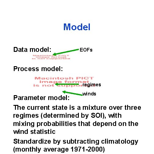
The Bayesian hierarchical approach Three levels of modelling: Data model: f(data | process, parameters) Process model: f(process | parameters) Parameter model: f(parameters) Use Bayes’ theorem to compute posterior f(process, parameters | data)

Some applications Data assimilation Satellite tracking Precipitation measurement Combination of data on different scales Image analysis Agricultural field trials

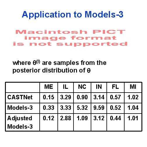
Application to Models-3 where (I) are samples from the posterior distribution of ME IL NC IN FL MI CASTNet 0. 15 3. 29 0. 90 3. 14 0. 57 1. 02 Models-3 0. 33 3. 33 5. 32 9. 59 0. 52 1. 04 Adjusted Models-3 0. 12 2. 88 1. 09 3. 12 0. 44 1. 01

Predictions

NCAR-GSP (IMAGe) Theme for 2005: Data Assimilation in the Geosciences

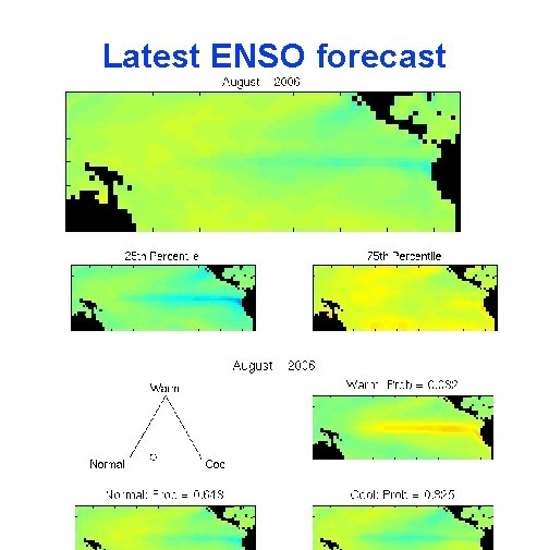
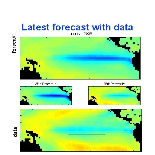
ENSO project El Niño/Southern Oscillation is driven by surface temperature in tropical Pacific Data 2 ox 2 o monthly SST anomalies at 2261 locations; zonal 10 m wind Previous work indicates EOFs of SST may develop in a Markovian fashion Forecast 7 months ahead uses data from Jan 70 through latest available. Cressie-Wikle-Berliner (http: //www. stat. ohio-state. edu/ ~sses/collab_enso. php)

Model Data model: EOFs Process model: regimes winds Parameter model: The current state is a mixture over three regimes (determined by SOI), with mixing probabilities that depend on the wind statistic Standardize by subtracting climatology (monthly average 1971 -2000)

Latest ENSO forecast

data forecast Latest forecast with data

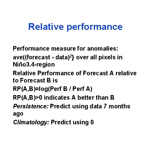
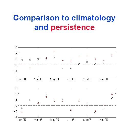
Relative performance Performance measure for anomalies: ave((forecast - data)2} over all pixels in Niño 3. 4 -region Relative Performance of Forecast A relative to Forecast B is RP(A, B)=log(Perf B / Perf A) RP(A, B)>0 indicates A better than B Persistence: Predict using data 7 months ago Climatology: Predict using 0

Comparison to climatology and persistence