Deterministic and Randomized Quicksort Andreas Klappenecker Overview Deterministic

Deterministic and Randomized Quicksort Andreas Klappenecker

Overview Deterministic Quicksort Modify Quicksort to obtain better asymptotic bound Linear-time median algorithm Randomized Quicksort

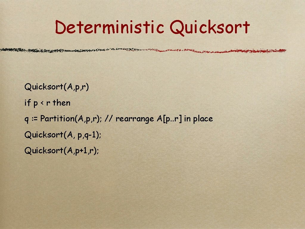
Deterministic Quicksort(A, p, r) if p < r then q : = Partition(A, p, r); // rearrange A[p. . r] in place Quicksort(A, p, q-1); Quicksort(A, p+1, r);

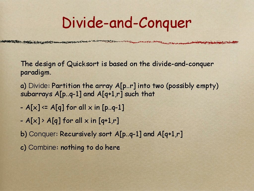
Divide-and-Conquer The design of Quicksort is based on the divide-and-conquer paradigm. a) Divide: Partition the array A[p. . r] into two (possibly empty) subarrays A[p. . q-1] and A[q+1, r] such that - A[x] <= A[q] for all x in [p. . q-1] - A[x] > A[q] for all x in [q+1, r] b) Conquer: Recursively sort A[p. . q-1] and A[q+1, r] c) Combine: nothing to do here

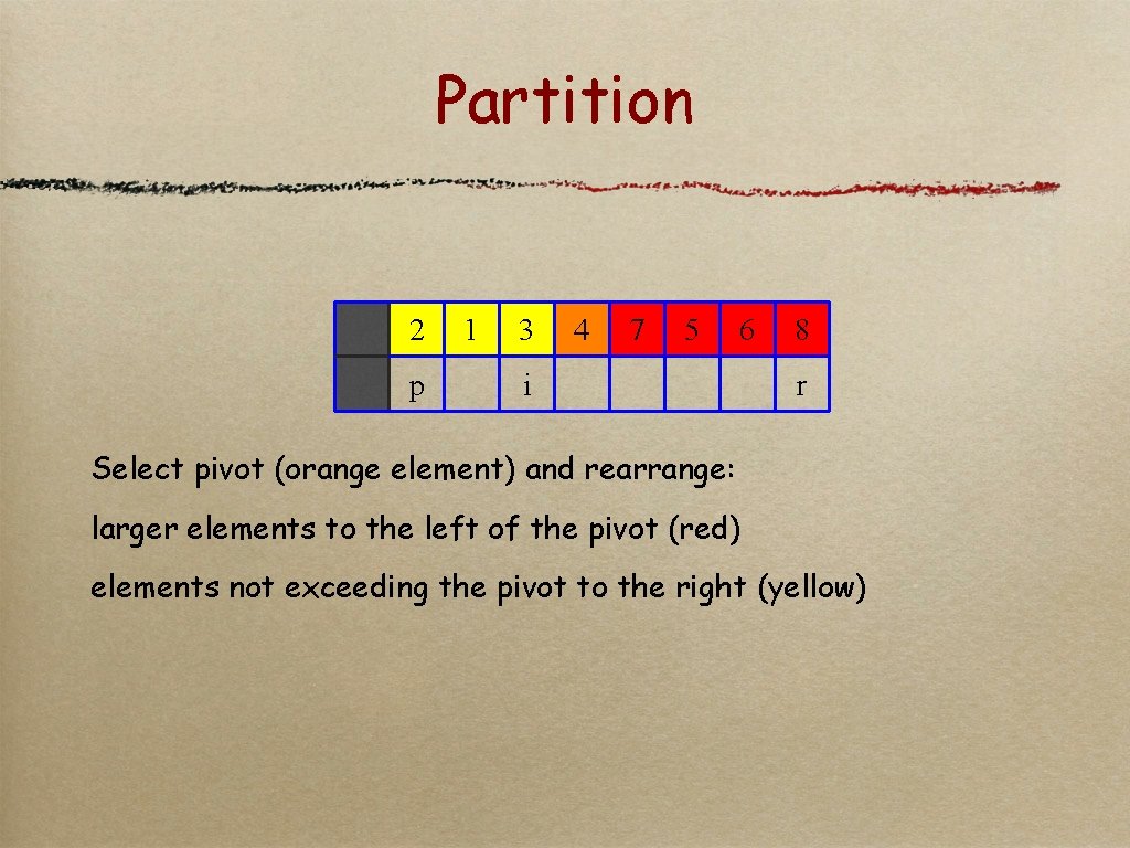
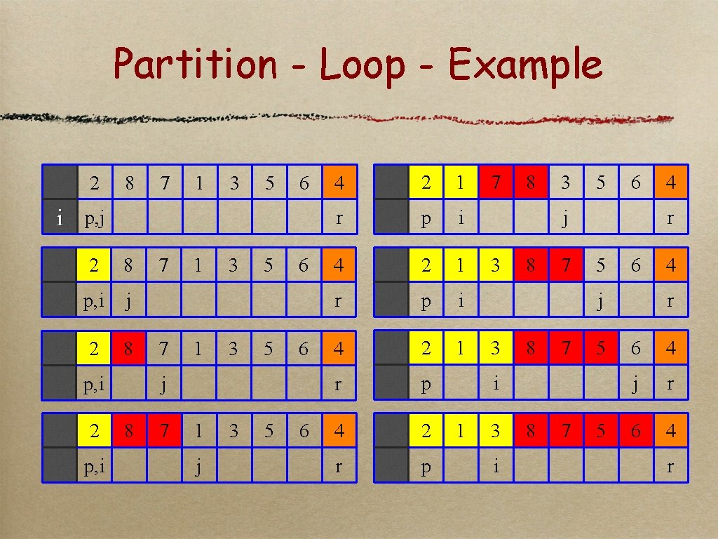
Partition 2 p 1 3 4 7 5 6 i 8 r Select pivot (orange element) and rearrange: larger elements to the left of the pivot (red) elements not exceeding the pivot to the right (yellow)

Partition(A, p, r) x : = A[r]; // select rightmost element as pivot i : = p-1; for j = p to r-1 do if A[j] <= x then i : = i+1; swap(A[i], A[j]); fi; od; swap(A[i+1], A[r]) return i+1; Throughout the for loop: • If p <= k <= i then A[k]<= x • If i+1<=k <= j-1 then A[k] > x • If k=r, then A[k] = x • A[j. . r-1] is unstructured

Partition - Loop - Example 2 8 7 1 3 5 6 i p, j 2 8 p, i 2 p, i 7 7 1 1 3 3 5 5 6 6 j 8 7 1 j 3 5 6 4 2 1 r p i 4 2 1 r p 4 2 r p 7 8 3 5 j 3 8 7 5 6 j 3 8 7 3 i 8 7 4 r 5 i 1 6 5 4 r 6 4 j r 6 4 r

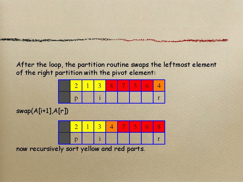
After the loop, the partition routine swaps the leftmost element of the right partition with the pivot element: 2 1 p 3 8 7 5 6 i 4 r swap(A[i+1], A[r]) 2 p 1 3 4 7 5 i now recursively sort yellow and red parts. 6 8 r

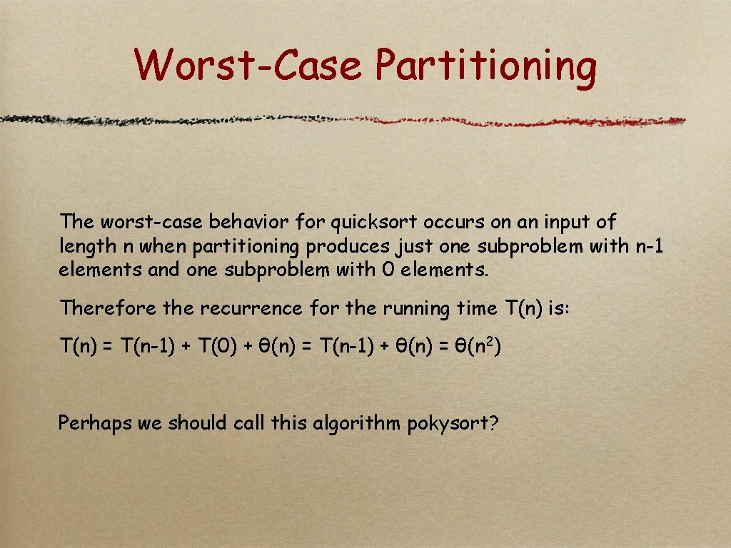
Worst-Case Partitioning The worst-case behavior for quicksort occurs on an input of length n when partitioning produces just one subproblem with n-1 elements and one subproblem with 0 elements. Therefore the recurrence for the running time T(n) is: T(n) = T(n-1) + T(0) + θ(n) = T(n-1) + θ(n) = θ(n 2) Perhaps we should call this algorithm pokysort?

“Better” Quicksort and Linear Median Algorithm

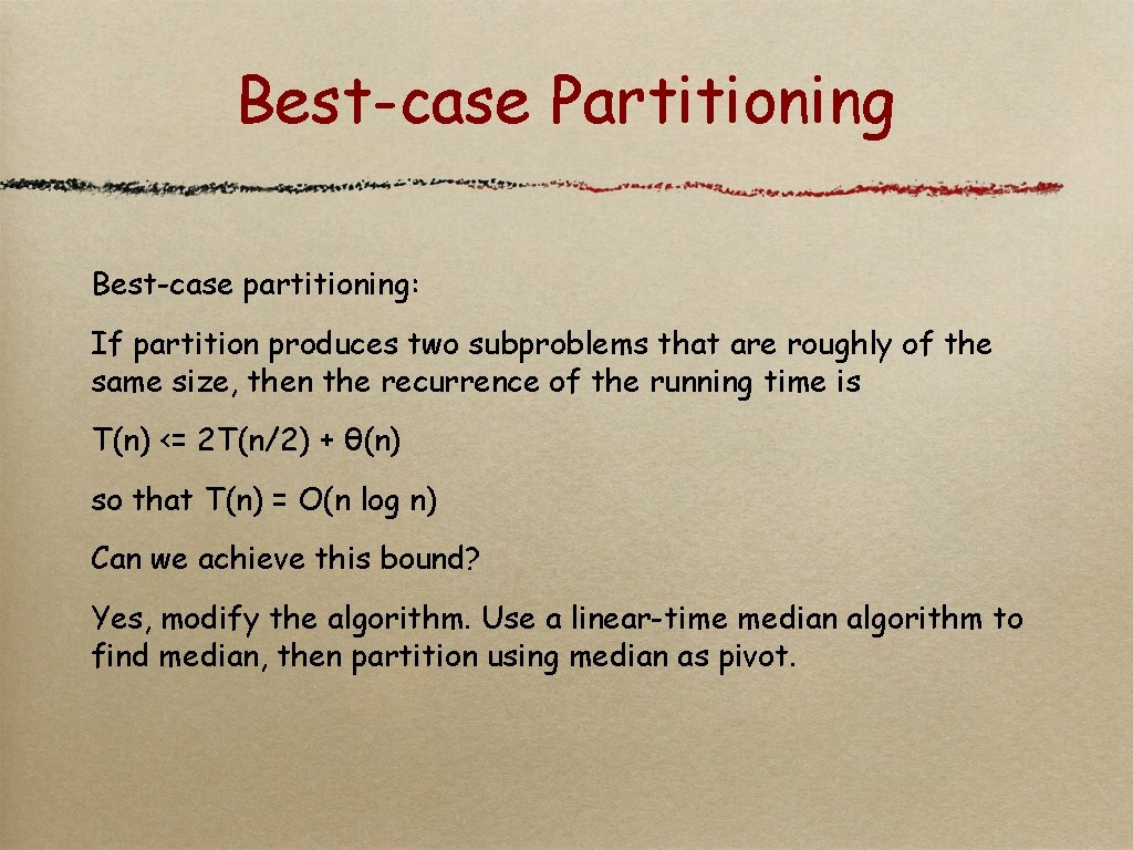
Best-case Partitioning Best-case partitioning: If partition produces two subproblems that are roughly of the same size, then the recurrence of the running time is T(n) <= 2 T(n/2) + θ(n) so that T(n) = O(n log n) Can we achieve this bound? Yes, modify the algorithm. Use a linear-time median algorithm to find median, then partition using median as pivot.

Linear Median Algorithm Let A[1. . n] be an array over a totally ordered domain. - Partition A into groups of 5 and find the median of each group. [You can do that with 6 comparisons] - Make an array U[1. . n/5] of the medians and find the median m of U by recursively calling the algorithm. - Partition the array A using the median-of-medians m to find the rank of m in A. If m is of larger rank than the median of A, eliminate all elements > m. If m is of smaller rank than the median of A, then eliminate all elements <= m. Repeat the search on the smaller array.

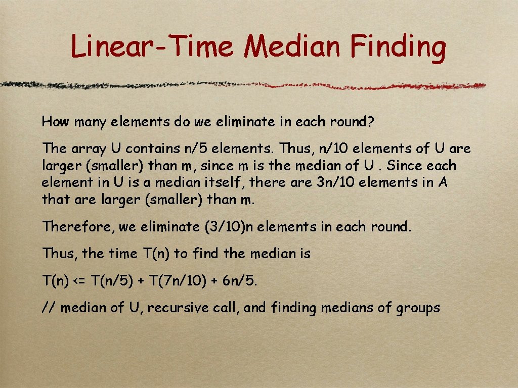
Linear-Time Median Finding How many elements do we eliminate in each round? The array U contains n/5 elements. Thus, n/10 elements of U are larger (smaller) than m, since m is the median of U. Since each element in U is a median itself, there are 3 n/10 elements in A that are larger (smaller) than m. Therefore, we eliminate (3/10)n elements in each round. Thus, the time T(n) to find the median is T(n) <= T(n/5) + T(7 n/10) + 6 n/5. // median of U, recursive call, and finding medians of groups

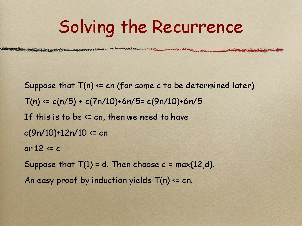
Solving the Recurrence Suppose that T(n) <= cn (for some c to be determined later) T(n) <= c(n/5) + c(7 n/10)+6 n/5= c(9 n/10)+6 n/5 If this is to be <= cn, then we need to have c(9 n/10)+12 n/10 <= cn or 12 <= c Suppose that T(1) = d. Then choose c = max{12, d}. An easy proof by induction yields T(n) <= cn.

Goal Achieved? We can accomplish that quicksort achieves O(n log n) running time, if we use the linear-time median finding algorithm to select the pivot element. Unfortunately, the constant in the big Oh expression becomes large, and quicksort looses some of its appeal. Is there a simpler solution?

Randomized Quicksort

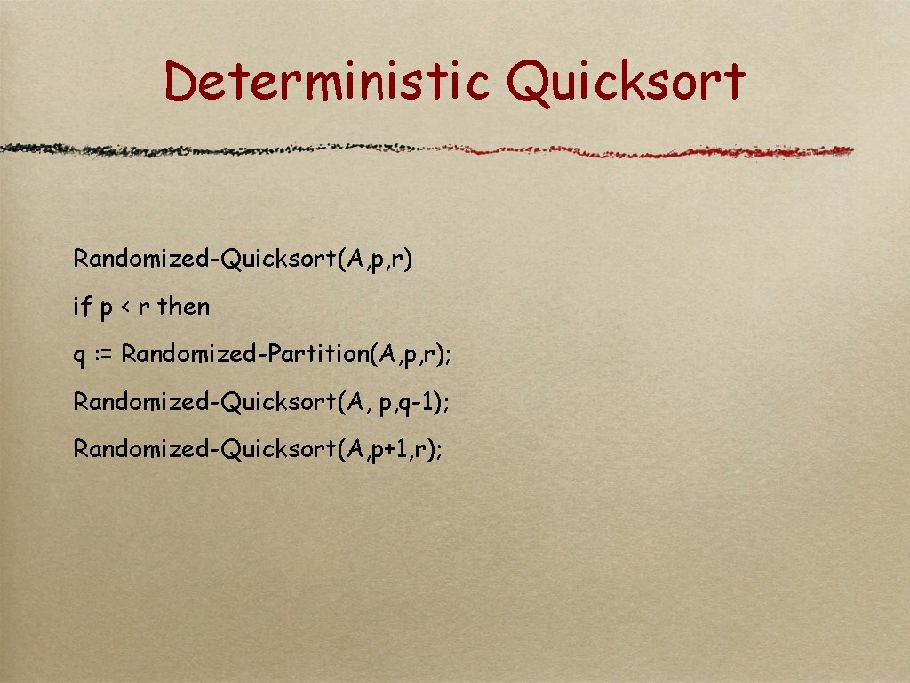
Deterministic Quicksort Randomized-Quicksort(A, p, r) if p < r then q : = Randomized-Partition(A, p, r); Randomized-Quicksort(A, p, q-1); Randomized-Quicksort(A, p+1, r);

Partition Randomized-Partition(A, p, r) i : = Random(p, r); swap(A[i], A[r]); Partition(A, p, r); Almost the same as Partition, but now the pivot element is not the rightmost element, but rather an element from A[p. . r] that is chosen uniformly at random.

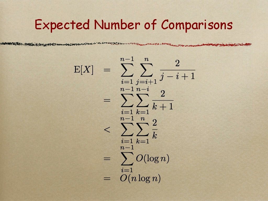
Goal The running time of quicksort depends mostly on the number of comparisons performed in all calls to the Randomized-Partition routine. Let X denote the random variable counting the number of comparisons in all calls to Randomized-Partition.

Notations Let zi denote the i-th smallest element of A[1. . n]. Thus A[1. . n] sorted is <z 1, z 2, . . . , zn >. Let Zij = {zi, . . . , zj} denote the set of elements between zi and zj, including these elements. Xij = I{ zi is compared to zj}. Thus, Xij is an indicator random variable for the event that the ith smallest and the j-th smallest elements of A are compared in an execution of quicksort.

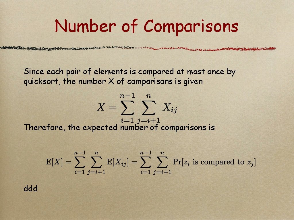
Number of Comparisons Since each pair of elements is compared at most once by quicksort, the number X of comparisons is given Therefore, the expected number of comparisons is ddd

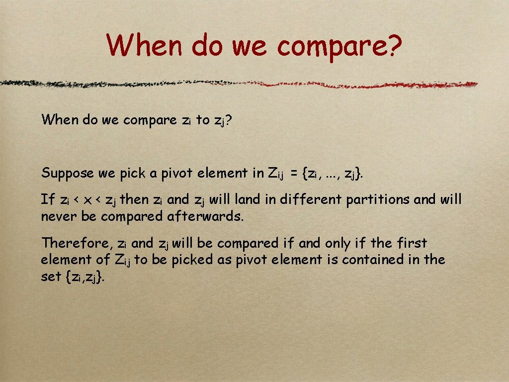
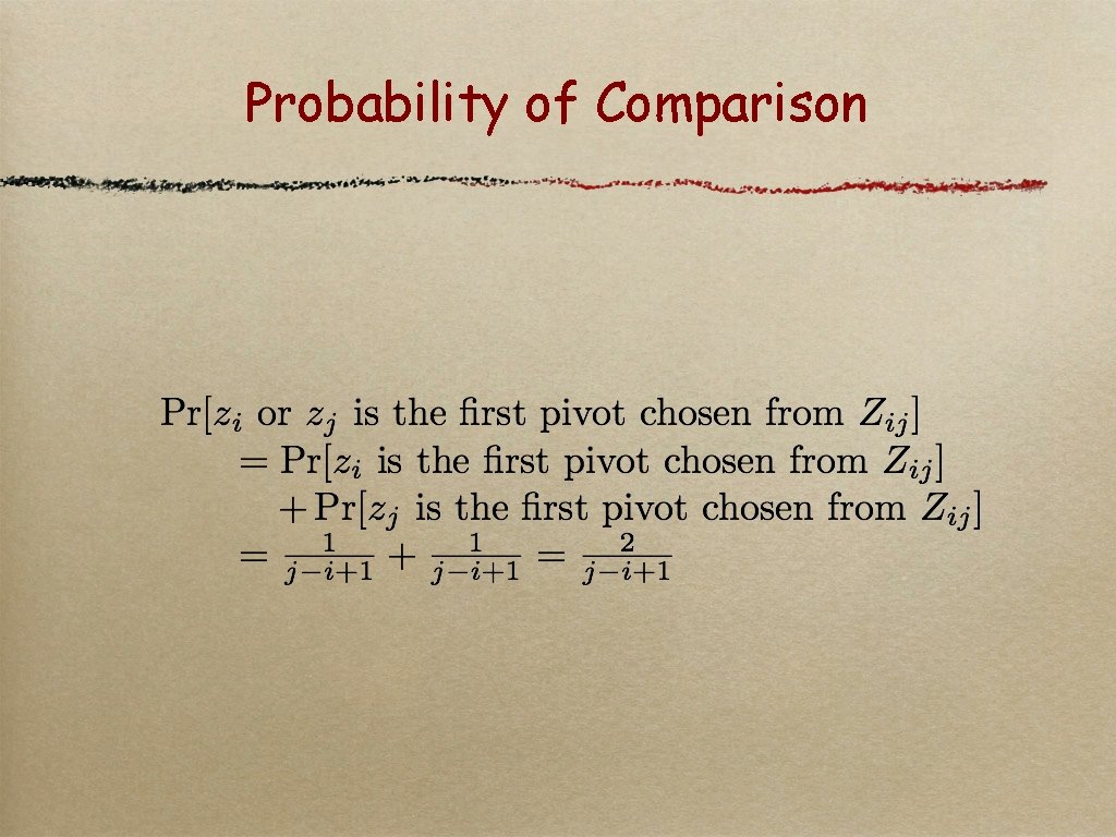
When do we compare? When do we compare zi to zj? Suppose we pick a pivot element in Zij = {zi, . . . , zj}. If zi < x < zj then zi and zj will land in different partitions and will never be compared afterwards. Therefore, zi and zj will be compared if and only if the first element of Zij to be picked as pivot element is contained in the set {zi, zj}.

Probability of Comparison

Expected Number of Comparisons

Conclusion It follows that the expected running time of Randomized. Quicksort is O(n log n). It is unlikely that this algorithm will choose a terribly unbalanced partition each time, so the performance is very good almost all the time.