Remaining Topics The vertexcover problem Bin Packing In

Remaining Topics

The vertex-cover problem

Bin Packing • In the bin packing problem, objects of different volumes must be packed into a finite number of bins or containers each of volume V in a way that minimizes the number of bins used. In computational complexity theory, it is a combinatorial NPhard problem. • There are many variations of this problem, such as 2 D packing, linear packing, packing by weight, packing by cost, and so on. • They have many applications, such as filling up containers, loading trucks with weight capacity constraints, creating file backups in removable media and technology mapping in Field -programmable gate array semiconductor chip design.

• The bin packing problem can also be seen as a special case of the cutting stock problem. • When the number of bins is restricted to 1 and each item is characterised by both a volume and a value, the problem of maximising the value of items that can fit in the bin is known as the knapsack problem. • Despite the fact that the bin packing problem has an NP-hard computational complexity, optimal solutions to very large instances of the problem can be produced with sophisticated algorithms. • In addition, many heuristics have been developed: for example, the first fit algorithm provides a fast but often nonoptimal solution, involving placing each item into the first bin in which it will fit. • It requires Θ(n log n) time, where n is the number of elements to be packed.

• The algorithm can be made much more effective by first sorting the list of elements into decreasing order (sometimes known as the first-fit decreasing algorithm), although this still does not guarantee an optimal solution, and for longer lists may increase the running time of the algorithm. • It is known, however, that there always exists at least one ordering of items that allows first-fit to produce an optimal solution. [1] • An interesting variant of bin packing that occurs in practice is when items can share space when packed into a bin. • Specifically, a set of items could occupy less space when packed together than the sum of their individual sizes.

• This variant is known as VM packing[2] since when virtual machines (VMs) are packed in a server, their total memory requirement could decrease due to pages shared by the VMs that need only be stored once. • If items can share space in arbitrary ways, the bin packing problem is hard to even approximate. • However, if the space sharing fits into a hierarchy, as is the case with memory sharing in virtual machines, the bin packing problem can be efficiently approximated.

Modular Arthmetic • In mathematics, modular arithmetic (sometimes called clock arithmetic) is a system of arithmetic for integers, where numbers "wrap around" upon reaching a certain value—the modulus.

• Modular arithmetic can be handled mathematically by introducing a congruence relation on the integers that is compatible with the operations of the ring of integers: addition, subtraction, and multiplication. For a positive integer n, two integers a and b are said to be congruent modulo n, written: • if their difference a − b is an integer multiple of n (or n divides a − b). The number n is called the modulus of the congruence.

• The properties that make this relation a congruence relation (respecting addition, subtraction, and multiplication) are the following. • If • And • then: • It should be noted that the above two properties would still hold if theory were expanded to include all real numbers, that is if were not necessarily all integers. The next property, however, would fail if these variables were not all integers:

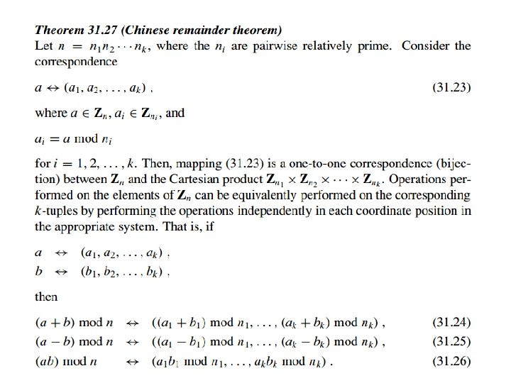
Chiness Theorem • The Chinese remainder theorem is a result about congruences in number theory and its generalizations in abstract algebra. It was first published in the 3 rd to 5 th centuries by Chinese mathematician Sun Tzu. • In its basic form, the Chinese remainder theorem will determine a number n that when divided by some given divisors leaves given remainders. • For example, what is the lowest number n that when divided by 3 leaves a remainder of 2, when divided by 5 leaves a remainder of 3, and when divided by 7 leaves a remainder of 2? • A common introductory example is a woman who tells a policeman that she lost her basket of eggs, and that if she makes three portions at a time out of it, she was left with 2, if she makes five portions at a time out of it, she was left with 3, and if she makes seven portions at a time out of it, she was left with 2. • She then asks the policeman what is the minimum number of eggs she must have had. The answer to both problems is 23.

• Suppose n 1, n 2, …, nk are positive integers that are pairwise coprime. Then, for any given sequence of integers a 1, a 2, …, ak, there exists an integer x solving the following system of simultaneous congruences.

Brute Force Technique: -

Optimization Problem • In mathematics and computer science, an optimization problem is the problem of finding the best solution from all feasible solutions. Optimization problems can be divided into two categories depending on whether the variables are continuous or discrete. • An optimization problem with discrete variables is known as a combinatorial optimization problem. In a combinatorial optimization problem, we are looking for an object such as an integer, permutation or graph from a finite (or possibly countable infinite) set.

Deterministic and Non Deterministic Problem A deterministic algorithm is an algorithm which, given a particular input, will always produce the same output, A nondeterministic algorithm is an algorithm that can exhibit different behaviors on different runs, as opposed to a deterministic algorithm A variety of factors can cause an algorithm to behave in a way which is not deterministic, or non-deterministic: 1. If it uses external state other than the input, such as user input, a global variable, a hardware timer value, a random value, or stored disk data. 2. If it operates in a way that is timing-sensitive, for example if it has multiple processors writing to the same data at the same time. In this case, the precise order in which each processor writes its data will affect the result. 3. If a hardware error causes its state to change in an unexpected way.

P And NP • P = set of problems that can be solved in polynomial time • NP = set of problems for which a solution can be verified in polynomial time. Or • NP (nondeterministic polynomial time) is the set of problems that can be solved in polynomial time by a nondeterministic computer • P NP • The big question: Does P = NP?

P and NP • The P versus NP problem is a major unsolved problem in computer science. Informally, it asks whether every problem whose solution can be quickly verified by a computer can also be quickly solved by a computer. • The informal term quickly used above means the existence of an algorithm for the task that runs in polynomial time. • The general class of questions for which some algorithm can provide an answer in polynomial time is called "class P" or just "P". • For some questions, there is no known way to find an answer quickly, but if one is provided with information showing what the answer is, it may be possible to verify the answer quickly. The class of questions for which an answer can be verified in polynomial time is called NP.

• Consider the subset sum problem, an example of a problem that is easy to verify, but whose answer may be difficult to compute. • Given a set of integers, does some nonempty subset of them sum to 0? For instance, does a subset of the set {− 2, − 3, 15, 14, 7, − 10} add up to 0? The answer "yes, because {− 2, − 3, − 10, 15} adds up to zero" can be quickly verified with three additions. • However, there is no known algorithm to find such a subset in polynomial time (there is one, however, in exponential time, which consists of 2 n-1 tries), and indeed such an algorithm can only exist if P = NP; hence this problem is in NP (quickly checkable) but not necessarily in P (quickly solvable).

• An answer to the P = NP question would determine whether problems that can be verified in polynomial time, like the subset-sum problem, can also be solved in polynomial time. • If it turned out that P ≠ NP, it would mean that there are problems in NP (such as NP-complete problems) that are harder to compute than to verify: they could not be solved in polynomial time, but the answer could be verified in polynomial time. • Aside from being an important problem in computational theory, a proof either way would have profound implications for mathematics, cryptography, algorithm research, artificial intelligence, game theory, multimedia processing and many other fields.

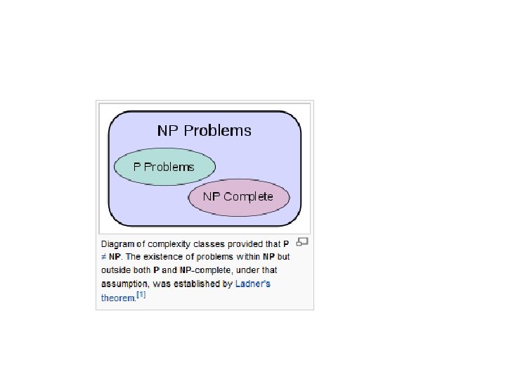
Relationship in P and NP • • The relation between the complexity classes P and NP is studied in computational complexity theory, the part of theory of computation dealing with the resources required during computation to solve a given problem. The most common resources are time (how many steps it takes to solve a problem) and space (how much memory it takes to solve a problem). In such analysis, a model of the computer for which time must be analyzed is required. Typically such models assume that the computer is deterministic (given the computer's present state and any inputs, there is only one possible action that the computer might take) and sequential (it performs actions one after the other). In this theory, the class P consists of all those decision problems that can be solved on a deterministic sequential machine in an amount of time that is polynomial in the size of the input; the class NP consists of all those decision problems whose positive solutions can be verified in polynomial time given the right information, or equivalently, whose solution can be found in polynomial time on a non-deterministic machine. Clearly, P ⊆ NP. Arguably the biggest open question in theoretical computer science concerns the relationship between those two classes: Is P equal to NP?

NP complete problem • • In computational complexity theory, the complexity class NP-complete (abbreviated NP-C or NPC) is a class of decision problems. A decision problem L is NP-complete if it is in the set of NP problems and also in the set of NP-hard problems. The abbreviation NP refers to "nondeterministic polynomial time. " Although any given solution to such a problem can be verified quickly, there is no known efficient way to locate a solution in the first place; indeed, the most notable characteristic of NP-complete problems is that no fast solution to them is known. That is, the time required to solve the problem using any currently known algorithm increases very quickly as the size of the problem grows. This means that the time required to solve even moderately sized versions of many of these problems can easily reach into the billions or trillions of years, using any amount of computing power available today. As a consequence, determining whether or not it is possible to solve these problems quickly, called the P versus NP problem, is one of the principal unsolved problems in computer science today. While a method for computing the solutions to NP-complete problems using a reasonable amount of time remains undiscovered, computer scientists and programmers still frequently encounter NP-complete problems are often addressed by using approximation algorithms.

• • • Formal overview NP-complete is a subset of NP, the set of all decision problems whose solutions can be verified in polynomial time; NP may be equivalently defined as the set of decision problems that can be solved in polynomial time on a nondeterministic Turing machine. A problem p in NP is also NP-complete if every other problem in NP can be transformed into p in polynomial time. NP-complete can also be used as an adjective: problems in the class NP-complete are known as NP-complete problems are studied because the ability to quickly verify solutions to a problem (NP) seems to correlate with the ability to quickly solve that problem (P). It is not known whether every problem in NP can be quickly solved—this is called the P = NP problem. But if any single problem in NP-complete can be solved quickly, then every problem in NP can also be quickly solved, because the definition of an NPcomplete problem states that every problem in NP must be quickly reducible to every problem in NP-complete (that is, it can be reduced in polynomial time). Because of this, it is often said that the NP-complete problems are harder or more difficult than NP problems in general.

NP Hard • NP-hard (Non-deterministic Polynomial-time hard), in computational complexity theory, is a class of problems that are, informally, "at least as hard as the hardest problems in NP". • A problem H is NP-hard if and only if there is an NP-complete problem L that is polynomial time Turing-reducible to H (i. e. , L TH). In other words, L can be solved in polynomial time by an oracle machine with an oracle for H. • Informally, we can think of an algorithm that can call such an oracle machine as a subroutine for solving H, and solves L in polynomial time, if the subroutine call takes only one step to compute. NP-hard problems may be of any type: decision problems, search problems, or optimization problems. • Example of an NP-hard problem is the optimization problem of finding the leastcost cyclic route through all nodes of a weighted graph. This is commonly known as the traveling salesman problem. • Another example of an NP-hard problem is the decision subset sum problem, which is this: given a set of integers, does any non-empty subset of them add up to zero? • That is a decision problem, and happens to be NP-complete.

There are decision problems that are NP-hard but not NPcomplete, for example the halting problem. This is the problem which asks "given a program and its input, will it run forever? " That's a yes/no question, so this is a decision problem.

NP-naming convention • NP-hard problems do not have to be elements of the complexity class NP, despite having NP as the prefix of their class name. The NP-naming system has some deeper sense, because the NP family is defined in relation to the class NP and the naming conventions in the Computational Complexity Theory. • NP Class of computational problems for which solutions can be verified by a non-deterministic Turing machine in polynomial time (or less). • NP-hard Class of problems which are at least as hard as the hardest problems in NP. Problems in NP-hard do not have to be elements of NP, indeed, they may not even be decision problems. • NP-complete Class of problems which contains the hardest problems in NP. Each element of NP-complete has to be an element of NP. • NP-easy At most as hard as NP, but not necessarily in NP, since they may not be decision problems. • NP-equivalent Exactly as difficult as the hardest problems in NP, but not necessarily in NP.

Resolving NP and P • We will see that NP-Complete problems are the “hardest” problems in NP: – If any one NP-Complete problem can be solved in polynomial time… – …then every NP-Complete problem can be solved in polynomial time… – …and in fact every problem in NP can be solved in polynomial time (which would show P = NP) – Thus: solve hamiltonian-cycle in O(n 100) time, you’ve proved that P = NP. Retire rich & famous.

Reduction • The crux of NP-Completeness is reducibility – Informally, a problem P can be reduced to another problem Q if any instance of P can be “easily rephrased” as an instance of Q, the solution to which provides a solution to the instance of P • What do you suppose “easily” means? • This rephrasing is called transformation – Intuitively: If P reduces to Q, P is “no harder to solve” than Q