Neural Networks References Artificial Intelligence for Games Artificial

Neural Networks References: • “Artificial Intelligence for Games” • "Artificial Intelligence: A new Synthesis"

History • In the 70’s it was *THE* approach to AI – Since then, not so much. • Although it has crept back into some apps. – It still has it’s uses. • Many different types of Neural Nets – (Multi-layer) Feed-forward (perceptron) – Hebbian – Recurrent

Overview • Givens: – A set of n training cases (each represented by a m-bit “binary string”) – The “correct” p-bit answer for each training case. • Supervised vs. Unsupervised • Process: – Train a neural network to “learn” the training cases. • Using the Neural Network. – When exposed to new (grey) inputs, it should pick the closest match. • Better than decision trees in this respect. • Basically: a classifier.

Example Application #1 • Modeling a enemy AI. • The AI can do one of these 4 actions: – – Go for cover Shoot nearest enemy Run away Idle • Training cases: – 50 sample play-throughs, 40 samples (2000 cases) with: • position of player (16 bits) • health of player (6 bits) • ammo-state of player (8 bits) – One of the following: • Supervised training: The action the AI *should* have taken. • Unsupervised training: A way to measure success (based on player/AI state)

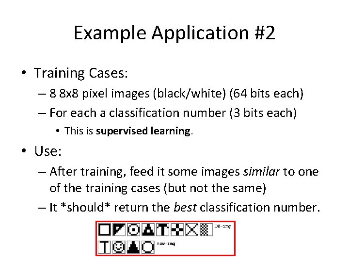
Example Application #2 • Training Cases: – 8 8 x 8 pixel images (black/white) (64 bits each) – For each a classification number (3 bits each) • This is supervised learning. • Use: – After training, feed it some images similar to one of the training cases (but not the same) – It *should* return the best classification number.

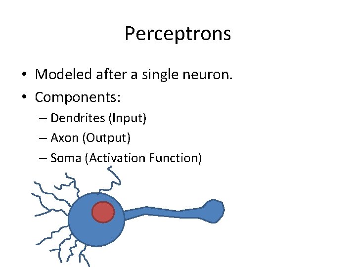
Perceptrons • Modeled after a single neuron. • Components: – Dendrites (Input) – Axon (Output) – Soma (Activation Function)

Part I: Perceptrons

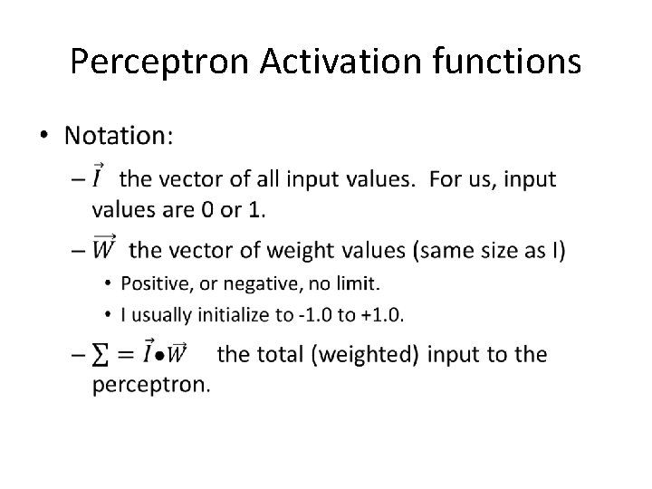
Perceptron Activation functions •

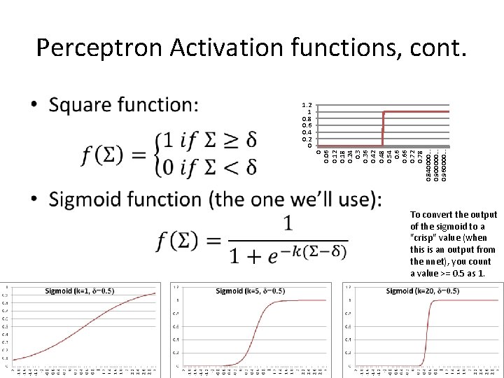
• 1. 2 1 0. 8 0. 6 0. 4 0. 2 0 0 0. 06 0. 12 0. 18 0. 24 0. 36 0. 42 0. 48 0. 54 0. 66 0. 72 0. 78 0. 840000. . . 0. 900000. . . 0. 960000. . . Perceptron Activation functions, cont. To convert the output of the sigmoid to a "crisp" value (when this is an output from the nnet), you count a value >= 0. 5 as 1.

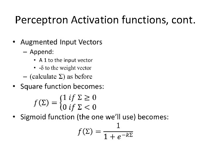
Perceptron Activation functions, cont. •

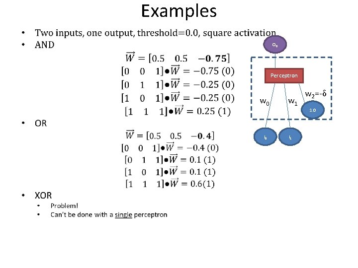
Examples • O 0 Perceptron w 0 I 0 w 1 I 1 w 2=-δ 1. 0

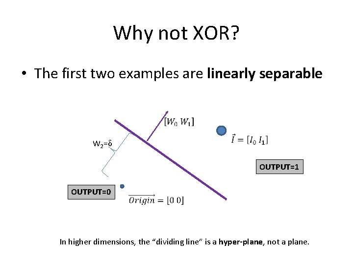
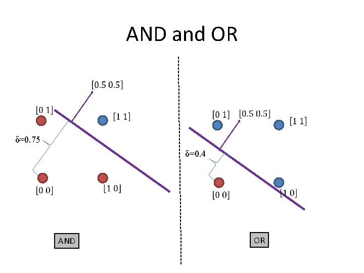
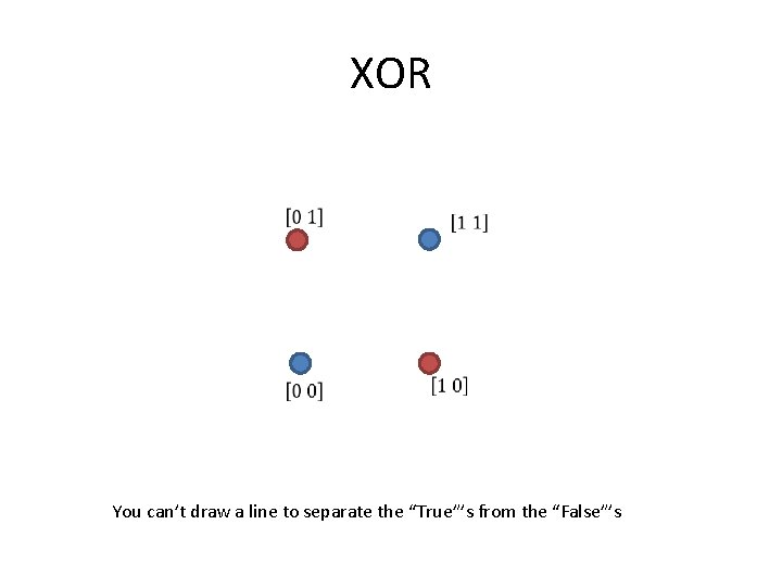
Why not XOR? • The first two examples are linearly separable W 2=δ OUTPUT=1 OUTPUT=0 In higher dimensions, the “dividing line” is a hyper-plane, not a plane.

AND and OR δ=0. 75 δ=0. 4 AND OR

XOR You can’t draw a line to separate the “True”’s from the “False”’s

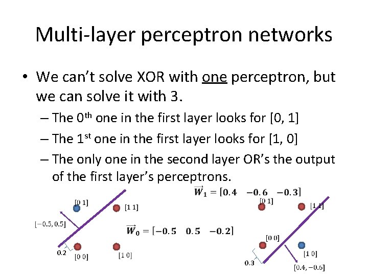
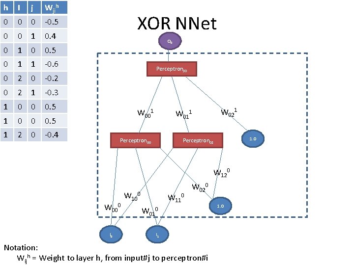
Multi-layer perceptron networks • We can’t solve XOR with one perceptron, but we can solve it with 3. – The 0 th one in the first layer looks for [0, 1] – The 1 st one in the first layer looks for [1, 0] – The only one in the second layer OR’s the output of the first layer’s perceptrons. 0. 2 0. 3

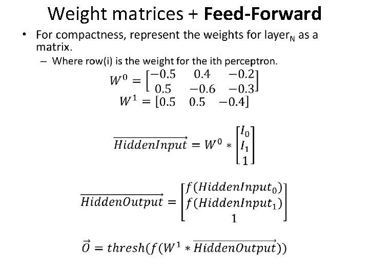
h I j Wjih 0 0 0 -0. 5 0 0 1 0. 4 0 1 0 0. 5 0 1 1 -0. 6 0 2 0 -0. 2 0 2 1 -0. 3 1 0 0 0. 5 1 2 0 -0. 4 XOR NNet O 0 Perceptron 10 W 001 W 021 W 011 Perceptron 00 1. 0 Perceptron 01 W 120 W 000 I 0 W 100 W 110 W 020 W 010 I 1 Notation: Wijh = Weight to layer h, from input#j to perceptron#i 1. 0

Weight matrices + Feed-Forward •

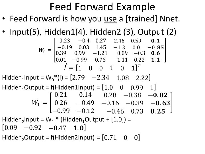
• Feed Forward Example

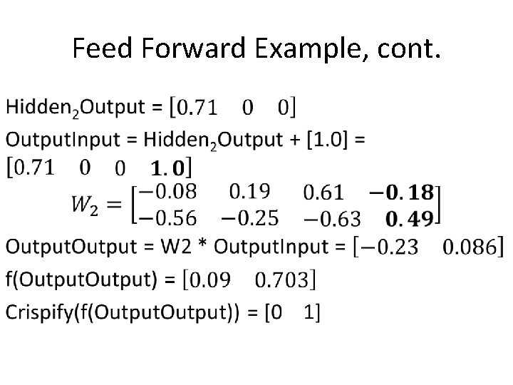
Feed Forward Example, cont. •

Part II: Training

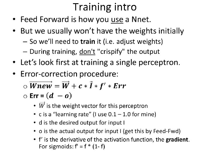
Training intro •

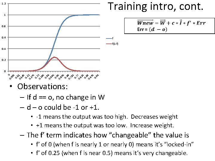
Training intro, cont. 1. 2 1 0. 8 0. 6 f f(1 -f) 0. 4 0. 2 0. 0 05 5 0. 11 0. 16 5 0. 2 27 5 0. 33 0. 38 5 0. 44 0. 49 5 0. 55 0. 60 5 0. 6 71 5 0. 77 0. 82 5 0. 88 0. 93 5 0. 99 0 • Observations: – If d == o, no change in W – d – o could be -1 or +1. • -1 means the output was too high. Decreases weight • +1 means the output was too low. Increase weight. – The f’ term indicates how “changeable” the value is • f’ of 0 (when f is nearly 1 or nearly 0) means it’s “locked-in” • f’ of 0. 25 (when f is near 0. 5) means it’s very changeable.

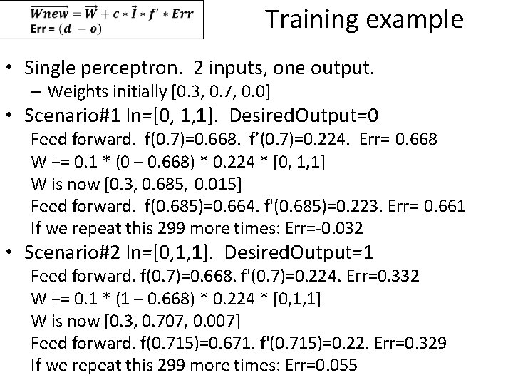
Training example • Single perceptron. 2 inputs, one output. – Weights initially [0. 3, 0. 7, 0. 0] • Scenario#1 In=[0, 1, 1]. Desired. Output=0 Feed forward. f(0. 7)=0. 668. f’(0. 7)=0. 224. Err=-0. 668 W += 0. 1 * (0 – 0. 668) * 0. 224 * [0, 1, 1] W is now [0. 3, 0. 685, -0. 015] Feed forward. f(0. 685)=0. 664. f'(0. 685)=0. 223. Err=-0. 661 If we repeat this 299 more times: Err=-0. 032 • Scenario#2 In=[0, 1, 1]. Desired. Output=1 Feed forward. f(0. 7)=0. 668. f'(0. 7)=0. 224. Err=0. 332 W += 0. 1 * (1 – 0. 668) * 0. 224 * [0, 1, 1] W is now [0. 3, 0. 707, 0. 007] Feed forward. f(0. 715)=0. 671. f'(0. 715)=0. 22. Err=0. 329 If we repeat this 299 more times: Err=0. 055

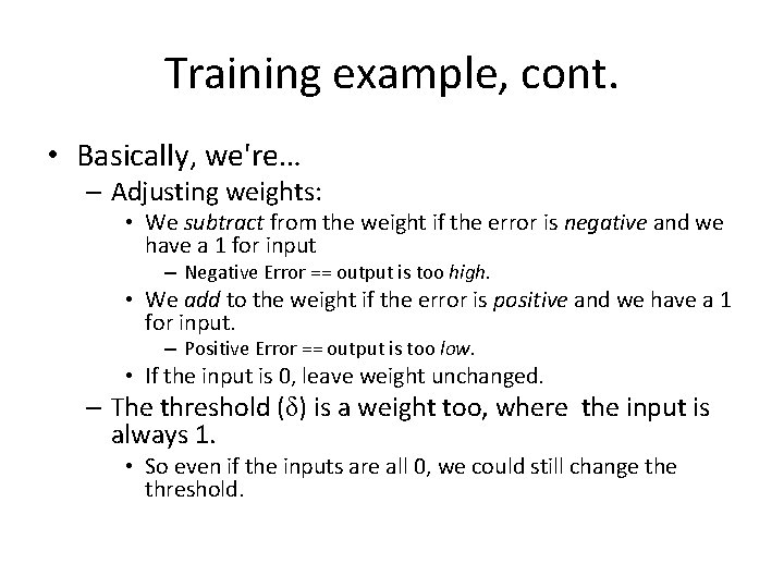
Training example, cont. • Basically, we're… – Adjusting weights: • We subtract from the weight if the error is negative and we have a 1 for input – Negative Error == output is too high. • We add to the weight if the error is positive and we have a 1 for input. – Positive Error == output is too low. • If the input is 0, leave weight unchanged. – The threshold (δ) is a weight too, where the input is always 1. • So even if the inputs are all 0, we could still change threshold.

Training intro, cont. • You repeatedly show examples, I – Perhaps in a random order • Weight values will stabilize at “correct” values. – *IF* the answers are linearly separable (like AND; unlike XOR) – If they aren’t it, will at least minimize the error.

Training Hidden Layers • A bit more complex… • The last weight matrix ("below" the output) is trained just as with a single perceptron – Treat the rows as the weight vectors. – The error is the difference between the desired output and actual output (not "crispified") – Row i in the weight matrix is considered the weight vector • For other matrices – The error is the error from the layer above weighted proportional to the (current) weight values feeding into that layer. • Assigning blame

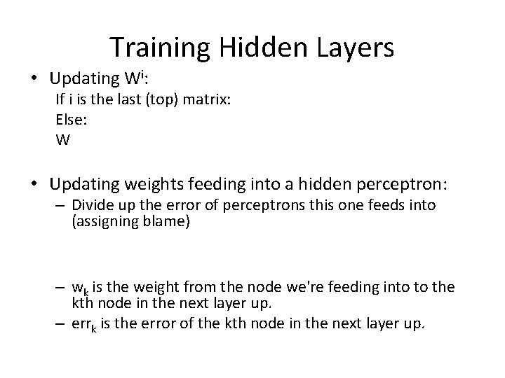
Training Hidden Layers • Updating Wi: If i is the last (top) matrix: Else: W • Updating weights feeding into a hidden perceptron: – Divide up the error of perceptrons this one feeds into (assigning blame) – wk is the weight from the node we're feeding into to the kth node in the next layer up. – errk is the error of the kth node in the next layer up.

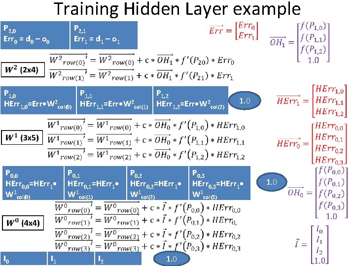
Training Hidden Layer example P 2, 0 Err 0 = d 0 – o 0 P 2, 1 Err 1 = d 1 – o 1 P 1, 0 P 1, 1 P 1, 2 HErr 1, 0=Err • W 2 col(0) HErr 1, 1=Err • W 2 col(1) HErr 1, 2=Err • W 2 col(2) 1. 0 P 0, 1 P 0, 2 P 0, 2 P 0, 3 HErr 0, 0=HErr 1 • HErr 0, 1=HErr 1 • HErr 0, 2=HErr 1 • HErr 0, 3=HErr 1 • W 1 col(0) W 1 col(1) W 1 col(2) W 1 col(3) I 0 I 1 I 2 1. 0