NATIONAL AND KAPODISTRIAN UIVERSITY OF ATHENS DEPARTMENT OF

NATIONAL AND KAPODISTRIAN UIVERSITY OF ATHENS DEPARTMENT OF INFORMATICS AND TELECOMMUNICATIONS GRADUATE PROGRAM DATA SCIENCE AND INFORMATION TECHNOLOGIES COURSE : BIOSTATISTICS NON-PARAMETRIC HYPOTHESIS TESTS DIONISIS LINARDATOS e-mail : dlinardatos@di. uoa. gr 5 DECEMBER 2019 1

Examples for hypothesis tests for normality and chi-square 2. Non-parametric hypothesis tests 3. Selection of the statistical test 1. 2

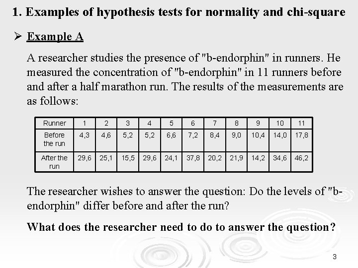
1. Examples of hypothesis tests for normality and chi-square Ø Example Α A researcher studies the presence of "b-endorphin" in runners. He measured the concentration of "b-endorphin" in 11 runners before and after a half marathon run. The results of the measurements are as follows: Runner 1 2 3 4 5 6 7 8 9 10 11 Before the run 4, 3 4, 6 5, 2 6, 6 7, 2 8, 4 9, 0 10, 4 14, 0 17, 8 After the run 29, 6 25, 1 15, 5 29, 6 24, 1 37, 8 20, 2 21, 9 14, 2 34, 6 46, 2 The researcher wishes to answer the question: Do the levels of "bendorphin" differ before and after the run? What does the researcher need to do to answer the question? 3

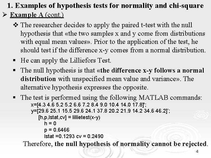
1. Examples of hypothesis tests for normality and chi-square Ø Example A (cont. ) v The researcher decides to apply the paired t-test with the null hypothesis that «the two samples x and y come from distributions with equal mean values» . Prior to the application of the test, he should test if the difference x-y comes from a normal distribution. § He can apply the Lilliefors Test. § The null hypothesis is that «the difference x-y follows a normal distribution with unspecified mean value and variance» . The alternative hypothesis expresses the opposite. § The test is performed using the following MATLAB commands: x=[4. 3 4. 6 5. 2 6. 6 7. 2 8. 4 9. 0 10. 4 14. 0 17. 8]'; y=[29. 6 25. 1 15. 5 29. 6 24. 1 37. 8 20. 2 21. 9 14. 2 34. 6 46. 2]’; [h, p, lstat, cv] = lillietest(x-y) h=0 p = 0. 6466 lstat =0. 1293 cv = 0. 2490 Therefore, the null hypothesis of normality cannot be rejected. 4

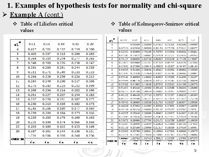
1. Examples of hypothesis tests for normality and chi-square Ø Example A (cont. ) v Table of Liliefors critical values v Table of Kolmogorov-Smirnov critical values 5

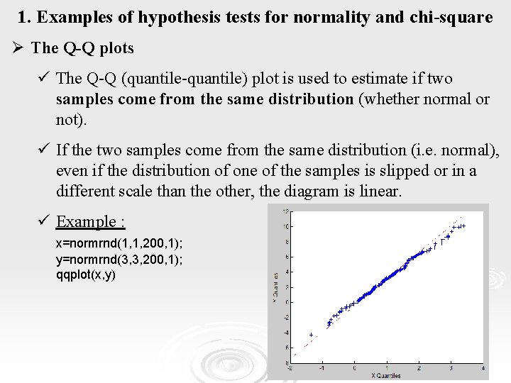
1. Examples of hypothesis tests for normality and chi-square Ø The Q-Q plots ü The Q-Q (quantile-quantile) plot is used to estimate if two samples come from the same distribution (whether normal or not). ü If the two samples come from the same distribution (i. e. normal), even if the distribution of one of the samples is slipped or in a different scale than the other, the diagram is linear. ü Example : x=normrnd(1, 1, 200, 1); y=normrnd(3, 3, 200, 1); qqplot(x, y) 6

1. Examples of hypothesis tests for normality and chi-square Ø The chi-square test is used when the variables are qualitative. Ø When we want to determine if there is a relation between two qualitative variables or when we want to examine whether a data set comes from a specific distribution, then we apply the chisquare test. Ø In either case, there are two categories of information we need : 1. the observed frequency of each cell of the contingency table and 2. the expected frequency of each cell which comes either from theory or through a known relationship. 7

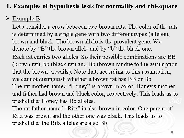
1. Examples of hypothesis tests for normality and chi-square Ø Example B Let's consider a cross between two brown rats. The color of the rats is determined by a single gene with two different types (alleles), brown and black. The brown allele is the prevalent gene. We denote by “B” the brown allele and by “b” the black one. Each rat carries two alleles. So their possible combinations are BB (brown rat), bb (black rat) and Bb (brown rat due to the assumption that the brown prevails). Note that, according to this assumption, we cannot distinguish whether a brown rat has BB or Bb. The rat mother named “Honey” is brown in color. Honey's mother and father had brown and black color, respectively. This leads us to predict that Honey has Bb alleles. The rat father named "Ritz" is also brown in color. One parent of Ritz was brown and the other one was black. This leads us to predict that the Ritz alleles are also Bb. 8

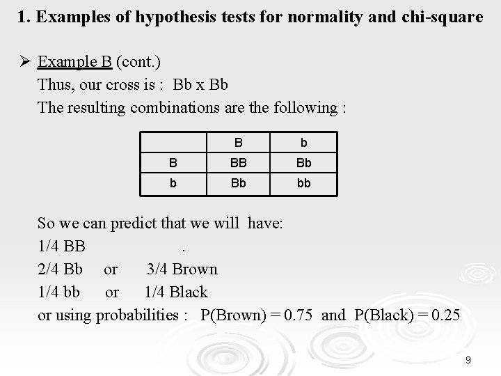
1. Examples of hypothesis tests for normality and chi-square Ø Example B (cont. ) Thus, our cross is : Bb x Bb The resulting combinations are the following : B b B BB Bb bb So we can predict that we will have: 1/4 BB. 2/4 Bb or 3/4 Brown 1/4 bb or 1/4 Black or using probabilities : P(Brown) = 0. 75 and P(Black) = 0. 25 9

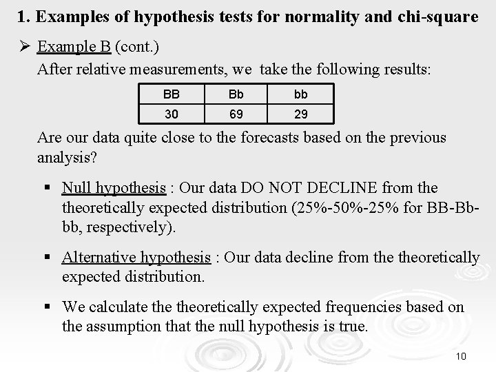
1. Examples of hypothesis tests for normality and chi-square Ø Example B (cont. ) After relative measurements, we take the following results: BB Bb bb 30 69 29 Are our data quite close to the forecasts based on the previous analysis? § Null hypothesis : Our data DO NOT DECLINE from theoretically expected distribution (25%-50%-25% for BB-Bbbb, respectively). § Alternative hypothesis : Our data decline from theoretically expected distribution. § We calculate theoretically expected frequencies based on the assumption that the null hypothesis is true. 10

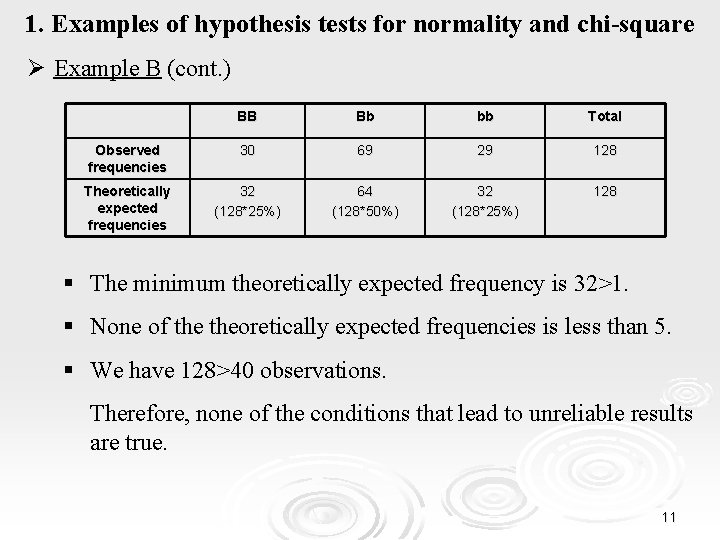
1. Examples of hypothesis tests for normality and chi-square Ø Example B (cont. ) BB Bb bb Total Observed frequencies 30 69 29 128 Theoretically expected frequencies 32 (128*25%) 64 (128*50%) 32 (128*25%) 128 § The minimum theoretically expected frequency is 32>1. § None of theoretically expected frequencies is less than 5. § We have 128>40 observations. Therefore, none of the conditions that lead to unreliable results are true. 11

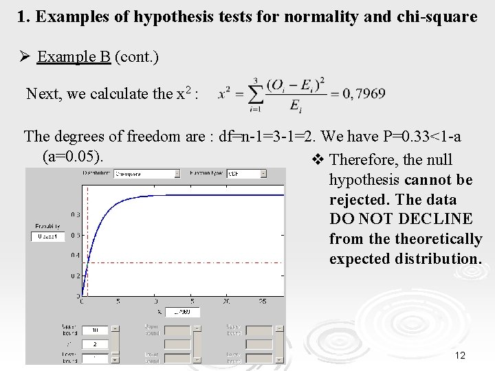
1. Examples of hypothesis tests for normality and chi-square Ø Example B (cont. ) Next, we calculate the x 2 : The degrees of freedom are : df=n-1=3 -1=2. We have P=0. 33<1 -a (a=0. 05). v Therefore, the null hypothesis cannot be rejected. The data DO NOT DECLINE from theoretically expected distribution. 12

1. Examples of hypothesis tests for normality and chi-square What to keep in mind when applying the chi-square tests? Ø The chi-square test provides unreliable results when: § The minimum theoretically expected value is smaller than 1. § More than the 20% of theoretically expected frequencies are smaller than 5. § We have less than 20 observations. § In the case of 2 x 2 contingency tables with 20 -40 observations, we have at least one of theoretically expected values less than 5. v When at least one of the above holds, we do not apply the chisquare test. Ø It is also emphasized that the chi-square tests are applied to the frequencies and not to the ratios or percentages derived from the frequencies. 13

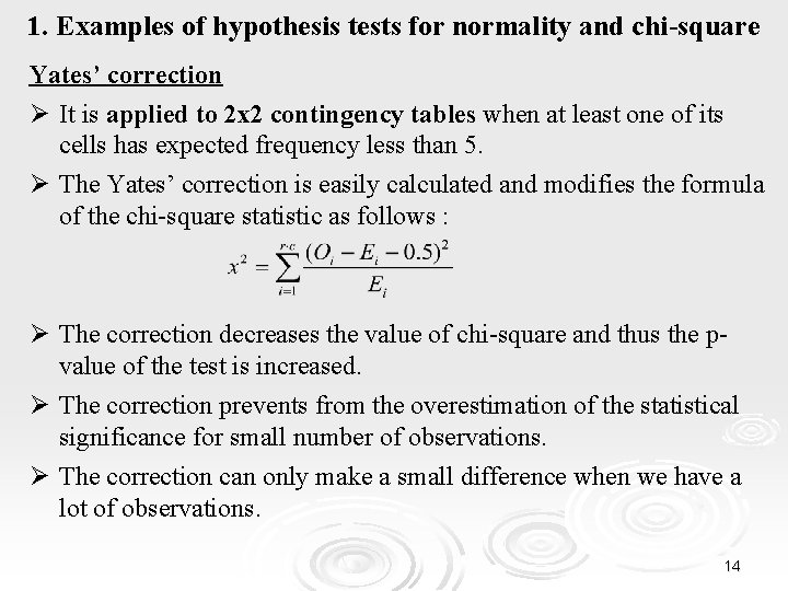
1. Examples of hypothesis tests for normality and chi-square Yates’ correction Ø It is applied to 2 x 2 contingency tables when at least one of its cells has expected frequency less than 5. Ø The Yates’ correction is easily calculated and modifies the formula of the chi-square statistic as follows : Ø The correction decreases the value of chi-square and thus the pvalue of the test is increased. Ø The correction prevents from the overestimation of the statistical significance for small number of observations. Ø The correction can only make a small difference when we have a lot of observations. 14

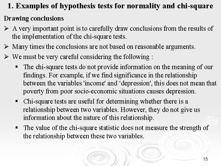
1. Examples of hypothesis tests for normality and chi-square Drawing conclusions Ø A very important point is to carefully draw conclusions from the results of the implementation of the chi-square tests. Ø Many times the conclusions are not based on reasonable arguments. Ø We must be very careful considering the following : § The chi-square tests do not provide information on the meaning of our findings. For example, if we find significance in the relationship between the variables 'income' and ‘depression', this does not mean that poverty from poor socio-economic situations causes depression. § Chi-square tests are useful for determining whethere is a relationship between two variables. However, they do not give us information about the nature of this relationship. § The value of the chi-square statistic does not measure the strength of the relationship between these two variables. 15

Examples for hypothesis tests for normality and chi-square 2. Non-parametric hypothesis tests 3. Selection of the statistical test 1. 16

2. Non-parametric hypothesis tests Ø Hypothesis tests are distinguished in : ü Parametric tests (Παραμετρικοί έλεγχοι) ü Non-parametric tests (Μη παραμετρικοί έλεγχοι) Ø The z-test and t-test are based on the assumption that the observations: § follow the normal distribution or § at least approximately follow the normal distribution or § follow the normal distribution after a transformation (i. e. logarithmic transformation) Ø The z-test and t-test are parametric tests. These are tests whose implementation is based on the existence of distribution parameters (i. e. N(0, 1), t(df), F(df)) 17

2. Non-parametric hypothesis tests Ø On the contrary, the non-parametric tests or distribution-free tests are the tests whose implementation does not require any assumption about distribution parameters. Ø The non-parametric procedures are less strong than the tests based on a particular distribution. Ø It is better using a stronger tool when its assumptions are satisfied, even approximately, than using a less strong tool with fewer assumptions. Ø For example, when a non-normal distribution can be transformed to a normal one by a logarithmic transformation, we prefer to use the transformed observations with a parametric method rather than to use the initial observations with a non-parametric method. 18

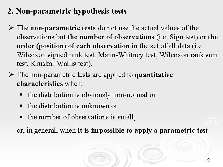
2. Non-parametric hypothesis tests Ø The non-parametric tests do not use the actual values of the observations but the number of observations (i. e. Sign test) or the order (position) of each observation in the set of all data (i. e. Wilcoxon signed rank test, Mann-Whitney test, Wilcoxon rank sum test, Kruskal-Wallis test). Ø The non-parametric tests are applied to quantitative characteristics when: § the distribution is obviously non-normal or § the distribution is unknown or § the number of observations is small, or, in general, when it is impossible to apply a parametric test. 19

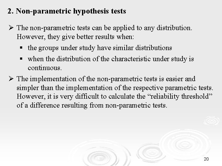
2. Non-parametric hypothesis tests Ø The non-parametric tests can be applied to any distribution. However, they give better results when: § the groups under study have similar distributions § when the distribution of the characteristic under study is continuous. Ø The implementation of the non-parametric tests is easier and simpler than the implementation of the respective parametric tests. However, it is very difficult to calculate the “reliability threshold” of a difference resulting from non-parametric tests. 20

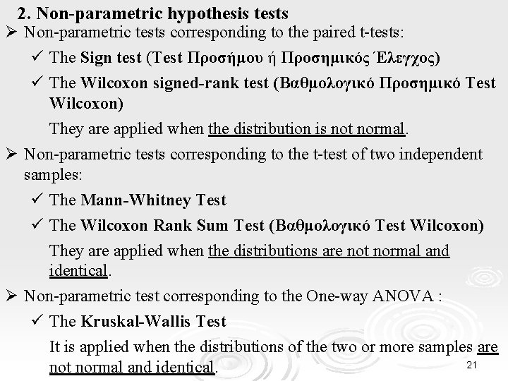
2. Non-parametric hypothesis tests Ø Non-parametric tests corresponding to the paired t-tests: ü The Sign test (Test Προσήμου ή Προσημικός Έλεγχος) ü The Wilcoxon signed-rank test (Βαθμολογικό Προσημικό Test Wilcoxon) They are applied when the distribution is not normal. Ø Non-parametric tests corresponding to the t-test of two independent samples: ü The Mann-Whitney Test ü The Wilcoxon Rank Sum Test (Βαθμολογικό Test Wilcoxon) They are applied when the distributions are not normal and identical. Ø Non-parametric test corresponding to the One-way ANOVA : ü The Kruskal-Wallis Test It is applied when the distributions of the two or more samples are 21 not normal and identical.

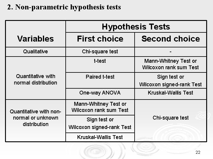
2. Non-parametric hypothesis tests Variables Qualitative Quantitative with normal distribution Quantitative with nonnormal or unknown distribution Hypothesis Tests First choice Second choice Chi-square test - t-test Mann-Whitney Test or Wilcoxon rank sum Test Paired t-test Sign test or Wilcoxon signed-rank Test Οne-way ANOVA Kruskal-Wallis Test Mann-Whitney Test or Wilcoxon rank sum Test Sign test or Wilcoxon signed-rank Test Chi-square test Kruskal-Wallis Test 22

2. Non-parametric hypothesis tests Ø The Wilcoxon Rank Sum Test ü The test is applied when: • we want to compare (that is, to see if there is any difference between them) two independent sets (groups) of observations • the two sets come from non-normal distributions or their distributions are unknown (that is the t-test cannot be applied). ü We assume that the two sets of observations are derived from continuous distributions of any form that are identical except from a possible sliding. 23

2. Non-parametric hypothesis tests Ø The Wilcoxon Rank Sum Test (cont. ) 1. We set the null hypothesis H 0: There IS NO DIFFERENCE between the two populations (their distributions have equal medians). 2. We set the alternative hypothesis H 1 : There is difference between the two populations (their distributions do not have equal medians). 3. We sort all observations (of both groups n 1 and n 2). ü We sort them from the smallest to the largest value (or vice versa). ü The order of each observation is its position in the sorted list, starting with 1 for the smallest observation. ü All equal values are sorted by the average value of the orders they occupy. 24

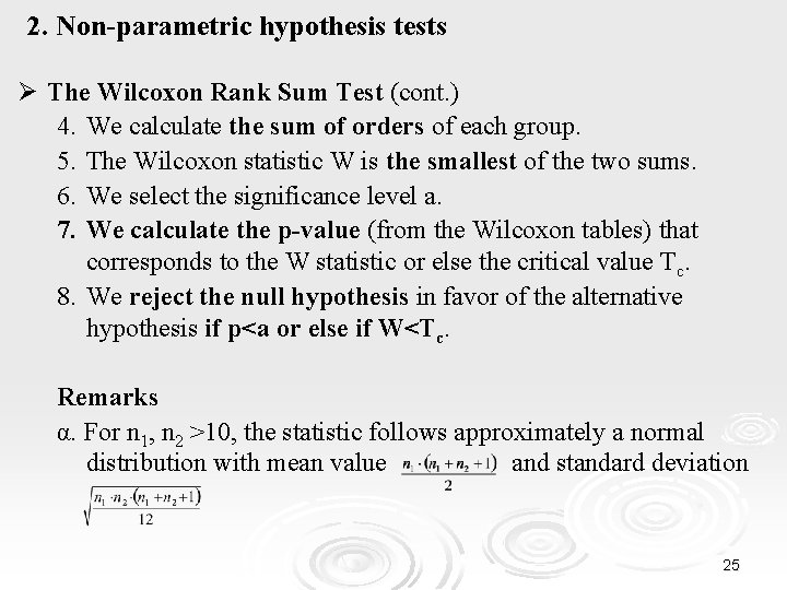
2. Non-parametric hypothesis tests Ø The Wilcoxon Rank Sum Test (cont. ) 4. We calculate the sum of orders of each group. 5. The Wilcoxon statistic W is the smallest of the two sums. 6. We select the significance level a. 7. We calculate the p-value (from the Wilcoxon tables) that corresponds to the W statistic or else the critical value Τc. 8. We reject the null hypothesis in favor of the alternative hypothesis if p<a or else if W<Τc. Remarks α. For n 1, n 2 >10, the statistic follows approximately a normal distribution with mean value and standard deviation 25

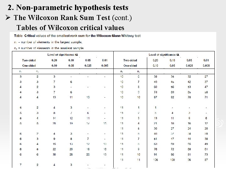
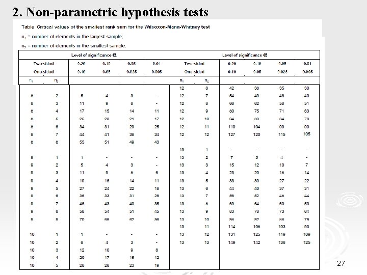
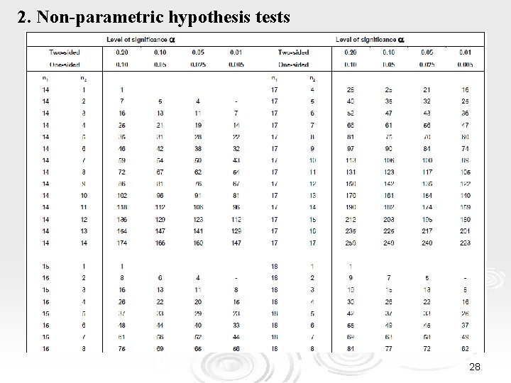
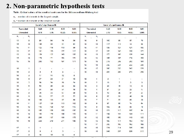
2. Non-parametric hypothesis tests Ø The Wilcoxon Rank Sum Test (cont. ) Tables of Wilcoxon critical values 26

2. Non-parametric hypothesis tests 27

2. Non-parametric hypothesis tests 28

2. Non-parametric hypothesis tests 29

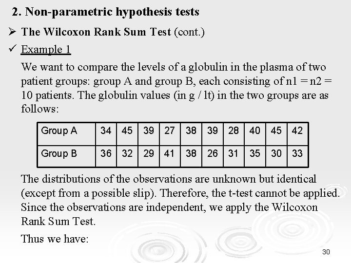
2. Non-parametric hypothesis tests Ø The Wilcoxon Rank Sum Test (cont. ) ü Example 1 We want to compare the levels of a globulin in the plasma of two patient groups: group A and group B, each consisting of n 1 = n 2 = 10 patients. The globulin values (in g / lt) in the two groups are as follows: Group A 34 45 39 27 38 39 28 40 45 42 Group B 36 32 29 41 38 26 31 35 30 33 The distributions of the observations are unknown but identical (except from a possible slip). Therefore, the t-test cannot be applied. Since the observations are independent, we apply the Wilcoxon Rank Sum Test. Thus we have: 30

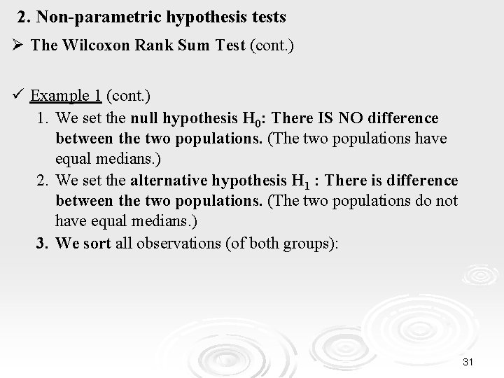
2. Non-parametric hypothesis tests Ø The Wilcoxon Rank Sum Test (cont. ) ü Example 1 (cont. ) 1. We set the null hypothesis H 0: There IS NO difference between the two populations. (The two populations have equal medians. ) 2. We set the alternative hypothesis H 1 : There is difference between the two populations. (The two populations do not have equal medians. ) 3. We sort all observations (of both groups): 31

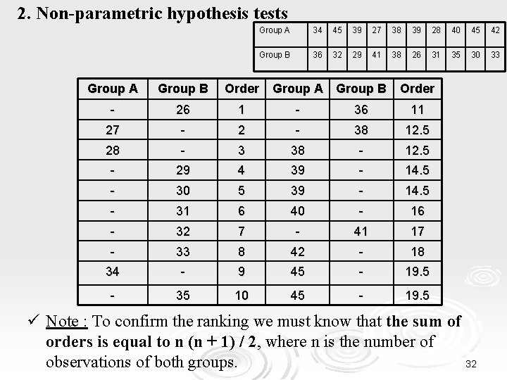
2. Non-parametric hypothesis tests Group A 34 45 39 27 38 39 28 40 45 42 Group B 36 32 29 41 38 26 31 35 30 33 Group A Group B Order - 26 1 - 36 11 27 - 2 - 38 12. 5 28 - 3 38 - 12. 5 - 29 4 39 - 14. 5 - 30 5 39 - 14. 5 - 31 6 40 - 16 - 32 7 - 41 17 - 33 8 42 - 18 34 - 9 45 - 19. 5 - 35 10 45 - 19. 5 ü Note : To confirm the ranking we must know that the sum of orders is equal to n (n + 1) / 2, where n is the number of observations of both groups. 32

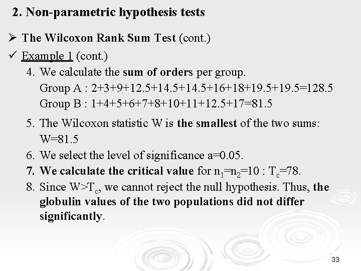
2. Non-parametric hypothesis tests Ø The Wilcoxon Rank Sum Test (cont. ) ü Example 1 (cont. ) 4. We calculate the sum of orders per group. Group A : 2+3+9+12. 5+14. 5+16+18+19. 5=128. 5 Group B : 1+4+5+6+7+8+10+11+12. 5+17=81. 5 5. The Wilcoxon statistic W is the smallest of the two sums: W=81. 5 6. We select the level of significance a=0. 05. 7. We calculate the critical value for n 1=n 2=10 : Tc=78. 8. Since W>Tc, we cannot reject the null hypothesis. Thus, the globulin values of the two populations did not differ significantly. 33

2. Non-parametric hypothesis tests Ø The Wilcoxon Rank Sum Test (cont. ) Matlab § The Statistics Toolbox provides the follow function to perform the Wilcoxon Rank Sum Test : Matlab function ranksum Hypothesis test Wilcoxon rank sum Test 34

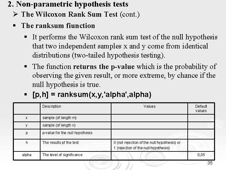
2. Non-parametric hypothesis tests Ø The Wilcoxon Rank Sum Test (cont. ) § The ranksum fiunction § It performs the Wilcoxon rank sum test of the null hypothesis that two independent samples x and y come from identical distributions (two-tailed hypothesis testing). § The function returns the p-value which is the probability of observing the given result, or more extreme, by chance if the null hypothesis is true. § [p, h] = ranksum(x, y, 'alpha', alpha) Description x sample (of length m) y sample (of length n) p p-value for the null hypothesis h The results pf the test alpha The level of significance Values Default values 0 (not rejection of the null hypothesis) or 1 (rejection of the null hypothesis) 0, 05 35

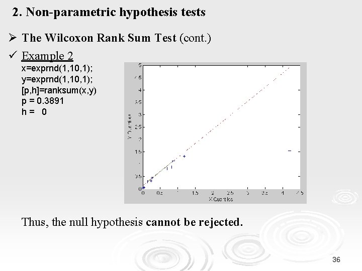
2. Non-parametric hypothesis tests Ø The Wilcoxon Rank Sum Test (cont. ) ü Example 2 x=exprnd(1, 10, 1); y=exprnd(1, 10, 1); [p, h]=ranksum(x, y) p = 0. 3891 h= 0 Thus, the null hypothesis cannot be rejected. 36

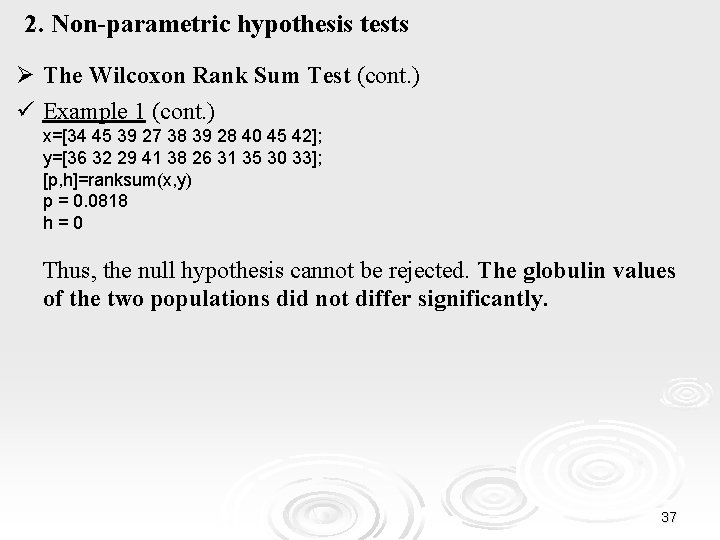
2. Non-parametric hypothesis tests Ø The Wilcoxon Rank Sum Test (cont. ) ü Example 1 (cont. ) x=[34 45 39 27 38 39 28 40 45 42]; y=[36 32 29 41 38 26 31 35 30 33]; [p, h]=ranksum(x, y) p = 0. 0818 h=0 Thus, the null hypothesis cannot be rejected. The globulin values of the two populations did not differ significantly. 37

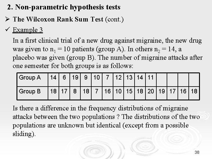
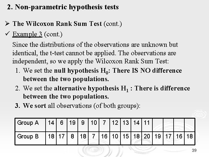
2. Non-parametric hypothesis tests Ø The Wilcoxon Rank Sum Test (cont. ) ü Example 3 In a first clinical trial of a new drug against migraine, the new drug was given to n 1 = 10 patients (group A). In others n 2 = 14, a placebo was given (group B). The number of migraine attacks after one semester for both groups is as follows: Group A 14 6 19 9 10 7 12 13 14 11 Group B 18 17 8 18 7 16 10 15 18 20 19 17 16 18 Is there a difference in the frequency distributions of migraine attacks between the two populations ? The distributions of the two populations are unknown but identical (except from a possible sliding). 38

2. Non-parametric hypothesis tests Ø The Wilcoxon Rank Sum Test (cont. ) ü Example 3 (cont. ) Since the distributions of the observations are unknown but identical, the t-test cannot be applied. The observations are independent, so we apply the Wilcoxon Rank Sum Test: 1. We set the null hypothesis H 0: There IS NO difference between the two populations. 2. We set the alternative hypothesis H 1 : There is difference between the two populations. 3. We sort all observations (of both groups): Group A 14 6 19 9 10 7 12 13 14 11 Group B 18 17 8 18 7 16 10 15 18 20 19 17 16 18 39

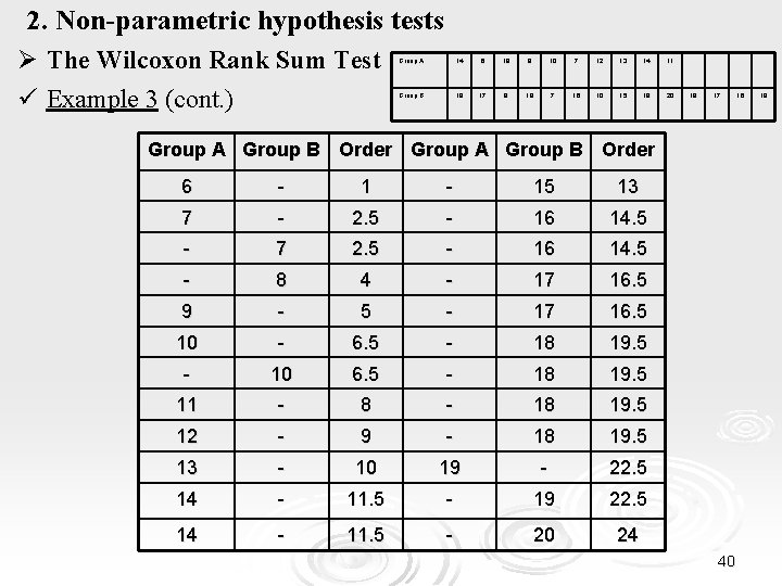
2. Non-parametric hypothesis tests Ø The Wilcoxon Rank Sum Test ü Example 3 (cont. ) Group A 14 6 19 9 10 7 12 13 14 11 Group B 18 17 8 18 7 16 10 15 18 20 19 17 Group A Group B Order 6 - 15 13 7 - 2. 5 - 16 14. 5 - 7 2. 5 - 16 14. 5 - 8 4 - 17 16. 5 9 - 5 - 17 16. 5 10 - 6. 5 - 18 19. 5 - 10 6. 5 - 18 19. 5 11 - 8 - 18 19. 5 12 - 9 - 18 19. 5 13 - 10 19 - 22. 5 14 - 11. 5 - 19 22. 5 14 - 11. 5 - 20 24 40 16 18

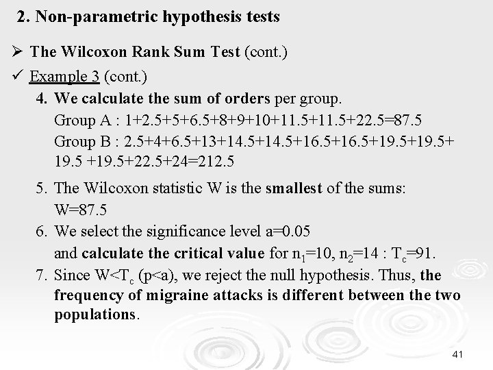
2. Non-parametric hypothesis tests Ø The Wilcoxon Rank Sum Test (cont. ) ü Example 3 (cont. ) 4. We calculate the sum of orders per group. Group A : 1+2. 5+5+6. 5+8+9+10+11. 5+22. 5=87. 5 Group B : 2. 5+4+6. 5+13+14. 5+16. 5+19. 5+ 19. 5 +19. 5+22. 5+24=212. 5 5. The Wilcoxon statistic W is the smallest of the sums: W=87. 5 6. We select the significance level a=0. 05 and calculate the critical value for n 1=10, n 2=14 : Tc=91. 7. Since W<Tc (p<a), we reject the null hypothesis. Thus, the frequency of migraine attacks is different between the two populations. 41

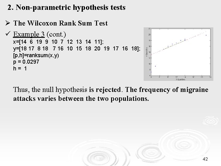
2. Non-parametric hypothesis tests Ø The Wilcoxon Rank Sum Test ü Example 3 (cont. ) x=[14 6 19 9 10 7 12 13 14 11]; y=[18 17 8 18 7 16 10 15 18 20 19 17 16 18]; [p, h]=ranksum(x, y) p = 0. 0297 h= 1 Thus, the null hypothesis is rejected. The frequency of migraine attacks varies between the two populations. 42

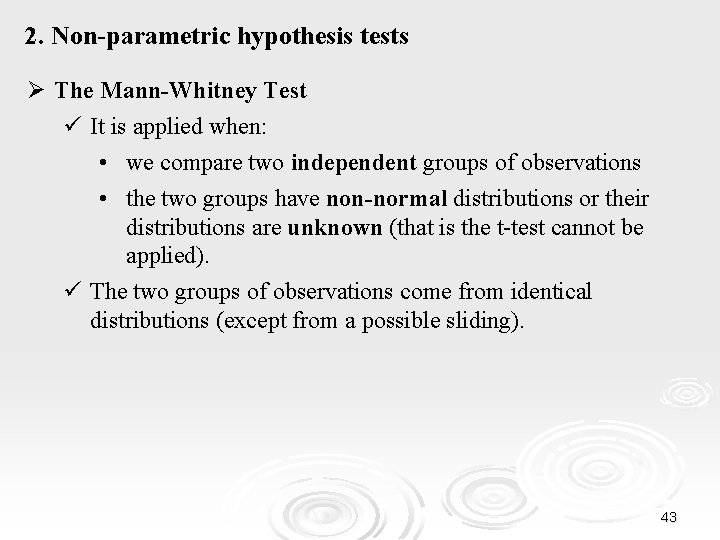
2. Non-parametric hypothesis tests Ø The Mann-Whitney Test ü It is applied when: • we compare two independent groups of observations • the two groups have non-normal distributions or their distributions are unknown (that is the t-test cannot be applied). ü The two groups of observations come from identical distributions (except from a possible sliding). 43

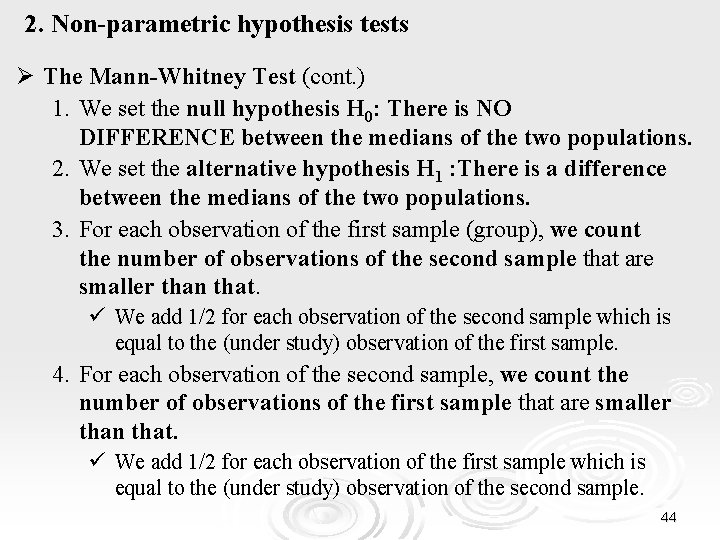
2. Non-parametric hypothesis tests Ø The Mann-Whitney Test (cont. ) 1. We set the null hypothesis H 0: There is NO DIFFERENCE between the medians of the two populations. 2. We set the alternative hypothesis H 1 : There is a difference between the medians of the two populations. 3. For each observation of the first sample (group), we count the number of observations of the second sample that are smaller than that. ü We add 1/2 for each observation of the second sample which is equal to the (under study) observation of the first sample. 4. For each observation of the second sample, we count the number of observations of the first sample that are smaller than that. ü We add 1/2 for each observation of the first sample which is equal to the (under study) observation of the second sample. 44

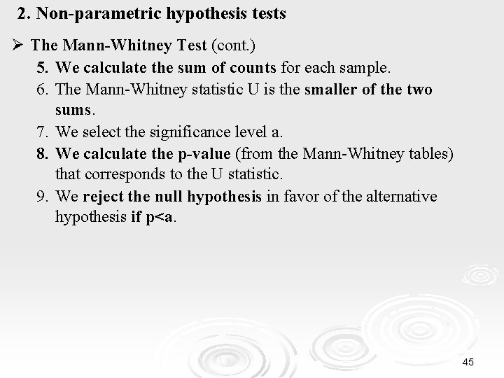
2. Non-parametric hypothesis tests Ø The Mann-Whitney Test (cont. ) 5. We calculate the sum of counts for each sample. 6. The Mann-Whitney statistic U is the smaller of the two sums. 7. We select the significance level a. 8. We calculate the p-value (from the Mann-Whitney tables) that corresponds to the U statistic. 9. We reject the null hypothesis in favor of the alternative hypothesis if p<a. 45

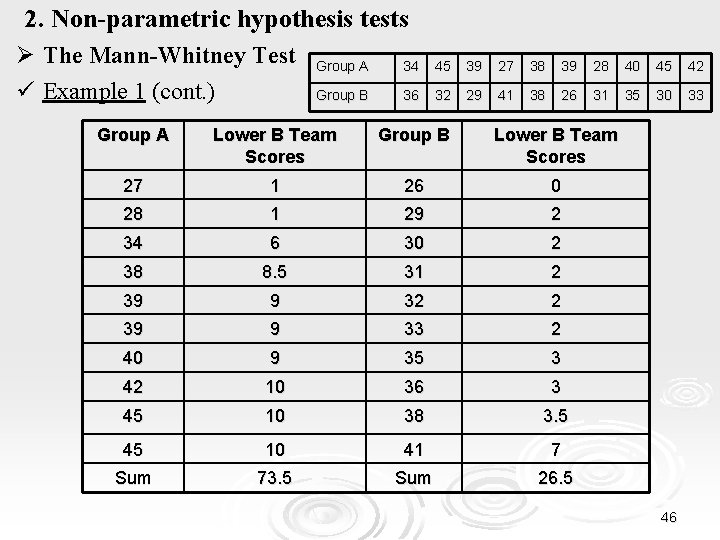
2. Non-parametric hypothesis tests Ø Τhe Mann-Whitney Test ü Example 1 (cont. ) Group A 34 45 39 27 38 39 28 40 45 42 Group B 36 32 29 41 38 26 31 35 30 33 Group A Lower B Team Scores Group B Lower B Team Scores 27 1 26 0 28 1 29 2 34 6 30 2 38 8. 5 31 2 39 9 32 2 39 9 33 2 40 9 35 3 42 10 36 3 45 10 38 3. 5 45 10 41 7 Sum 73. 5 Sum 26. 5 46

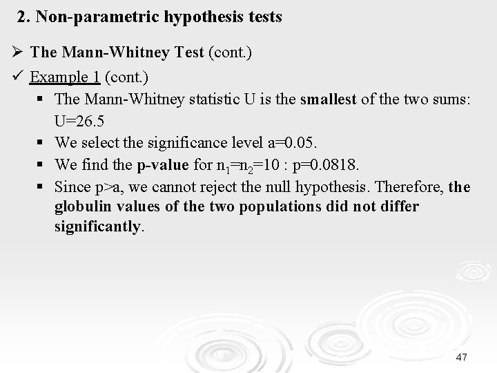
2. Non-parametric hypothesis tests Ø The Mann-Whitney Test (cont. ) ü Example 1 (cont. ) § The Mann-Whitney statistic U is the smallest of the two sums: U=26. 5 § We select the significance level a=0. 05. § We find the p-value for n 1=n 2=10 : p=0. 0818. § Since p>a, we cannot reject the null hypothesis. Therefore, the globulin values of the two populations did not differ significantly. 47

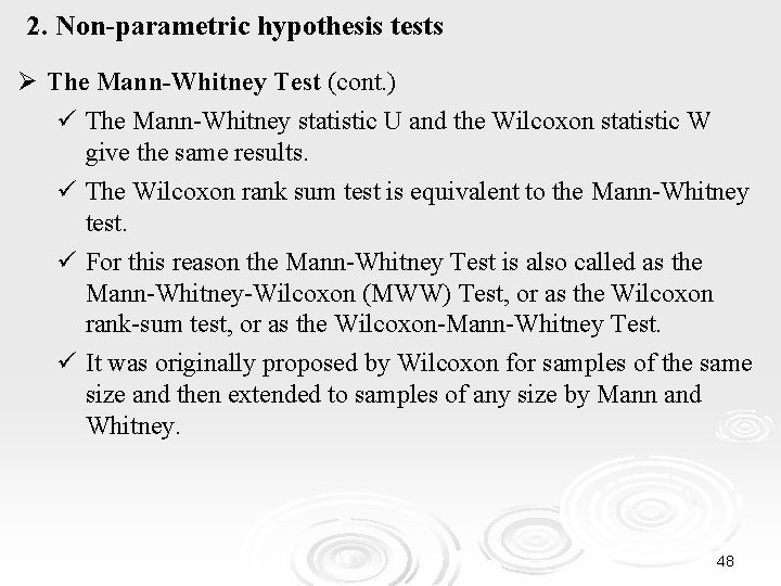
2. Non-parametric hypothesis tests Ø The Mann-Whitney Test (cont. ) ü The Mann-Whitney statistic U and the Wilcoxon statistic W give the same results. ü The Wilcoxon rank sum test is equivalent to the Mann-Whitney test. ü For this reason the Mann-Whitney Test is also called as the Mann-Whitney-Wilcoxon (MWW) Test, or as the Wilcoxon rank-sum test, or as the Wilcoxon-Mann-Whitney Test. ü It was originally proposed by Wilcoxon for samples of the same size and then extended to samples of any size by Mann and Whitney. 48

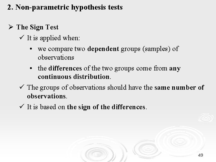
2. Non-parametric hypothesis tests Ø The Sign Test ü It is applied when: • we compare two dependent groups (samples) of observations • the differences of the two groups come from any continuous distribution. ü The groups of observations should have the same number of observations. ü It is based on the sign of the differences. 49

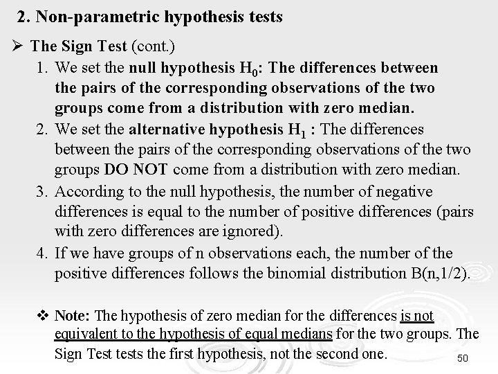
2. Non-parametric hypothesis tests Ø The Sign Test (cont. ) 1. We set the null hypothesis H 0: The differences between the pairs of the corresponding observations of the two groups come from a distribution with zero median. 2. We set the alternative hypothesis H 1 : The differences between the pairs of the corresponding observations of the two groups DO NOT come from a distribution with zero median. 3. According to the null hypothesis, the number of negative differences is equal to the number of positive differences (pairs with zero differences are ignored). 4. If we have groups of n observations each, the number of the positive differences follows the binomial distribution B(n, 1/2). v Note: The hypothesis of zero median for the differences is not equivalent to the hypothesis of equal medians for the two groups. The Sign Test tests the first hypothesis, not the second one. 50

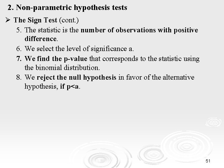
2. Non-parametric hypothesis tests Ø The Sign Test (cont. ) 5. The statistic is the number of observations with positive difference. 6. We select the level of significance a. 7. We find the p-value that corresponds to the statistic using the binomial distribution. 8. We reject the null hypothesis in favor of the alternative hypothesis, if p<a. 51

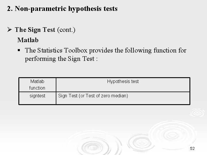
2. Non-parametric hypothesis tests Ø The Sign Test (cont. ) Matlab § The Statistics Toolbox provides the following function for performing the Sign Test : Matlab function signtest Hypothesis test Sign Test (or Test of zero median) 52

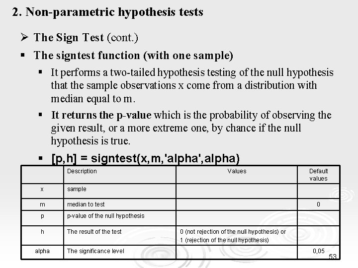
2. Non-parametric hypothesis tests Ø The Sign Test (cont. ) § The signtest function (with one sample) § It performs a two-tailed hypothesis testing of the null hypothesis that the sample observations x come from a distribution with median equal to m. § It returns the p-value which is the probability of observing the given result, or a more extreme one, by chance if the null hypothesis is true. § [p, h] = signtest(x, m, 'alpha', alpha) Description x sample m median to test p p-value of the null hypothesis h The result of the test alpha The significance level Values Default values 0 0 (not rejection of the null hypothesis) or 1 (rejection of the null hypothesis) 0, 05 53

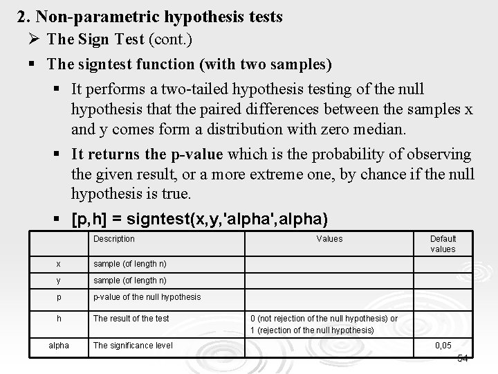
2. Non-parametric hypothesis tests Ø The Sign Test (cont. ) § The signtest function (with two samples) § It performs a two-tailed hypothesis testing of the null hypothesis that the paired differences between the samples x and y comes form a distribution with zero median. § It returns the p-value which is the probability of observing the given result, or a more extreme one, by chance if the null hypothesis is true. § [p, h] = signtest(x, y, 'alpha', alpha) Description x sample (of length n) y sample (of length n) p p-value of the null hypothesis h The result of the test alpha The significance level Values Default values 0 (not rejection of the null hypothesis) or 1 (rejection of the null hypothesis) 0, 05 54

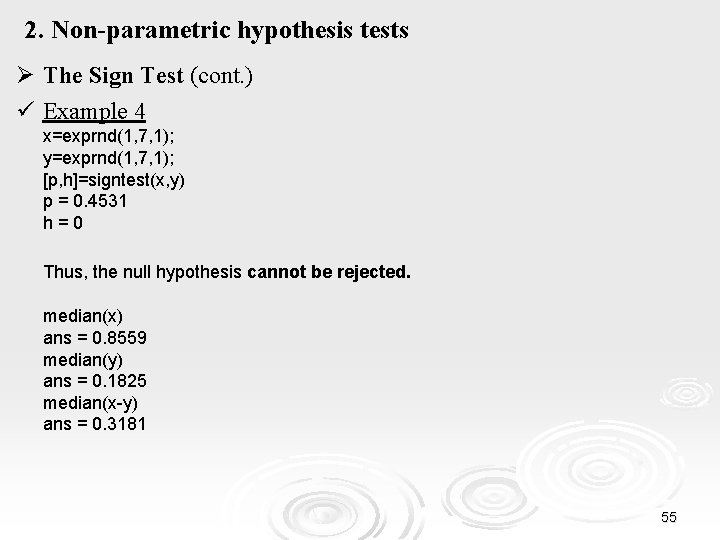
2. Non-parametric hypothesis tests Ø The Sign Test (cont. ) ü Example 4 x=exprnd(1, 7, 1); y=exprnd(1, 7, 1); [p, h]=signtest(x, y) p = 0. 4531 h=0 Thus, the null hypothesis cannot be rejected. median(x) ans = 0. 8559 median(y) ans = 0. 1825 median(x-y) ans = 0. 3181 55

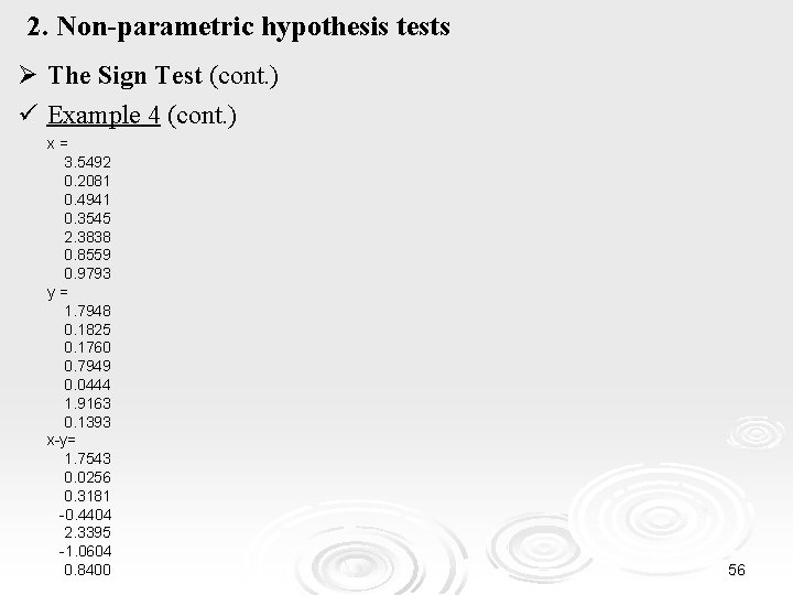
2. Non-parametric hypothesis tests Ø The Sign Test (cont. ) ü Example 4 (cont. ) x= 3. 5492 0. 2081 0. 4941 0. 3545 2. 3838 0. 8559 0. 9793 y= 1. 7948 0. 1825 0. 1760 0. 7949 0. 0444 1. 9163 0. 1393 x-y= 1. 7543 0. 0256 0. 3181 -0. 4404 2. 3395 -1. 0604 0. 8400 56

2. Non-parametric hypothesis tests Ø The Wilcoxon Signed-Rank Test ü It is applied when: • we compare two dependent groups (samples) of observations • the differences of the two groups come from any continuous distribution. ü The groups of observations should have the same number of observations. ü It is an improvement on the Sign Test. It takes into account the degree to which the pairs of the observations differ. ü It assumes that the population distribution of the paired differences is symmetric. 57

2. Non-parametric hypothesis tests Ø The Wilcoxon Signed-Rank Test (cont. ) 1. We set the null hypothesis H 0: The differences between the pairs of the corresponding observations of the two groups come from a distribution with zero median. 2. We set the alternative hypothesis H 1 : The differences between the pairs of the corresponding observations of the two groups DO NOT come from a distribution with zero median. 3. We calculate the differences of the corresponding observations. ü The differences maybe positive, negative or zero. ü We ignore the zero differences from further processing. v Note: The hypothesis of zero median for the differences is not equivalent to the hypothesis of equal medians for the two groups. The Wilcoxon Signed-Rank Test tests the first hypothesis, not the second 58 one.

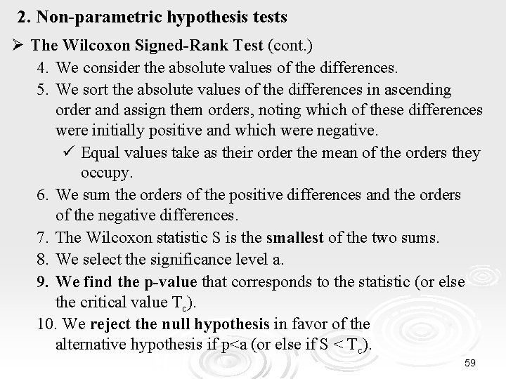
2. Non-parametric hypothesis tests Ø The Wilcoxon Signed-Rank Test (cont. ) 4. We consider the absolute values of the differences. 5. We sort the absolute values of the differences in ascending order and assign them orders, noting which of these differences were initially positive and which were negative. ü Equal values take as their order the mean of the orders they occupy. 6. We sum the orders of the positive differences and the orders of the negative differences. 7. The Wilcoxon statistic S is the smallest of the two sums. 8. We select the significance level a. 9. We find the p-value that corresponds to the statistic (or else the critical value Tc). 10. We reject the null hypothesis in favor of the alternative hypothesis if p<a (or else if S < Tc). 59

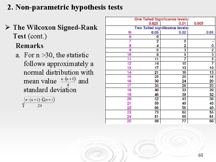
2. Non-parametric hypothesis tests Ø The Wilcoxon Signed-Rank Test (cont. ) Remarks a. For n >30, the statistic follows approximately a normal distribution with mean value and standard deviation 60

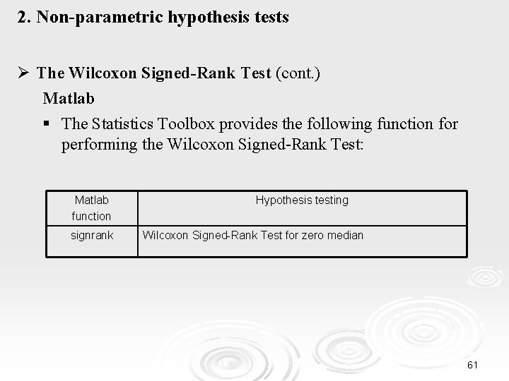
2. Non-parametric hypothesis tests Ø The Wilcoxon Signed-Rank Test (cont. ) Matlab § The Statistics Toolbox provides the following function for performing the Wilcoxon Signed-Rank Test: Matlab function signrank Hypothesis testing Wilcoxon Signed-Rank Test for zero median 61

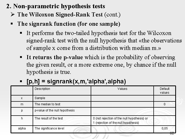
2. Non-parametric hypothesis tests Ø The Wilcoxon Signed-Rank Test (cont. ) § The signrank function (for one sample) § It performs the two-tailed hypothesis test for the Wilcoxon signed-rank test with the null hypothesis that «the observations of sample x come from a distribution with median m. » § It returns the p-value which is the probability of observing the given result, or a more extreme one, by chance if the null hypothesis is true. § [p, h] = signrank(x, m, 'alpha', alpha) Description x Sample m The median to test p p-value of the null hypothesis h The result of the test alpha The significance level Values Default values 0 0 (not rejection of the null hypothesis) or 1 (rejection of the null hypothesis) 0, 05 62

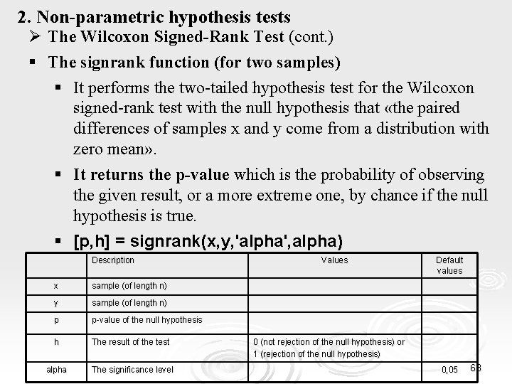
2. Non-parametric hypothesis tests Ø The Wilcoxon Signed-Rank Test (cont. ) § The signrank function (for two samples) § It performs the two-tailed hypothesis test for the Wilcoxon signed-rank test with the null hypothesis that «the paired differences of samples x and y come from a distribution with zero mean» . § It returns the p-value which is the probability of observing the given result, or a more extreme one, by chance if the null hypothesis is true. § [p, h] = signrank(x, y, 'alpha', alpha) Description x sample (of length n) y sample (of length n) p p-value of the null hypothesis h The result of the test alpha The significance level Values Default values 0 (not rejection of the null hypothesis) or 1 (rejection of the null hypothesis) 0, 05 63

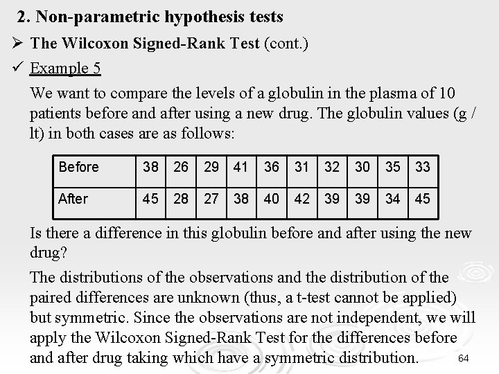
2. Non-parametric hypothesis tests Ø The Wilcoxon Signed-Rank Test (cont. ) ü Example 5 We want to compare the levels of a globulin in the plasma of 10 patients before and after using a new drug. The globulin values (g / lt) in both cases are as follows: Before 38 26 29 41 36 31 32 30 35 33 After 45 28 27 38 40 42 39 39 34 45 Is there a difference in this globulin before and after using the new drug? The distributions of the observations and the distribution of the paired differences are unknown (thus, a t-test cannot be applied) but symmetric. Since the observations are not independent, we will apply the Wilcoxon Signed-Rank Test for the differences before 64 and after drug taking which have a symmetric distribution.

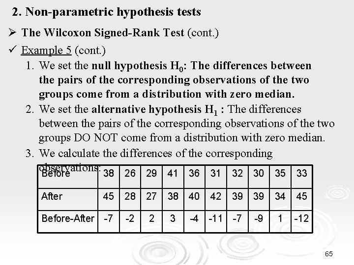
2. Non-parametric hypothesis tests Ø The Wilcoxon Signed-Rank Test (cont. ) ü Example 5 (cont. ) 1. We set the null hypothesis H 0: The differences between the pairs of the corresponding observations of the two groups come from a distribution with zero median. 2. We set the alternative hypothesis H 1 : The differences between the pairs of the corresponding observations of the two groups DO NOT come from a distribution with zero median. 3. We calculate the differences of the corresponding observations: Before 38 26 29 41 36 31 32 30 35 33 After 45 28 27 38 40 42 39 39 34 45 Before-After -7 -2 2 3 -4 -11 -7 -9 1 -12 65

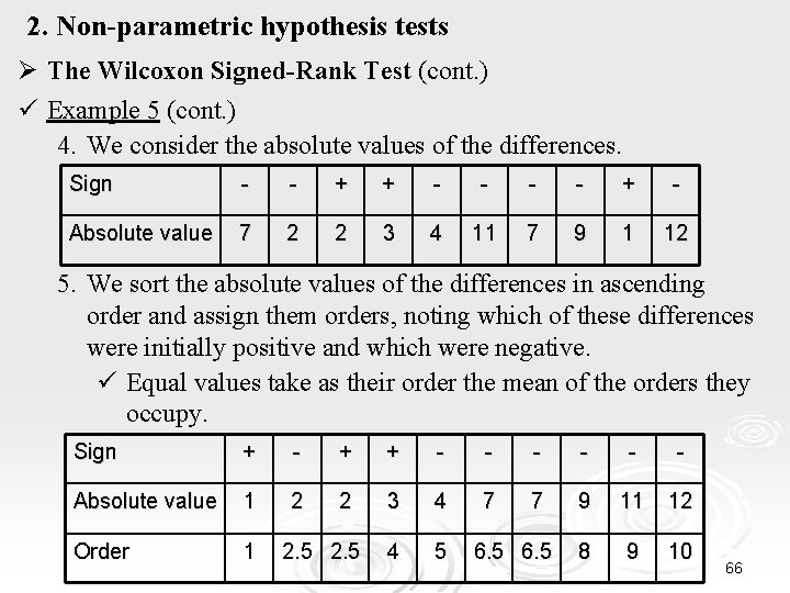
2. Non-parametric hypothesis tests Ø The Wilcoxon Signed-Rank Test (cont. ) ü Example 5 (cont. ) 4. We consider the absolute values of the differences. Sign - - + + - - + - Absolute value 7 2 2 3 4 11 7 9 1 12 5. We sort the absolute values of the differences in ascending order and assign them orders, noting which of these differences were initially positive and which were negative. ü Equal values take as their order the mean of the orders they occupy. Sign + - + + - - - Absolute value 1 2 2 3 4 7 7 9 11 12 Order 1 4 5 8 9 10 2. 5 66

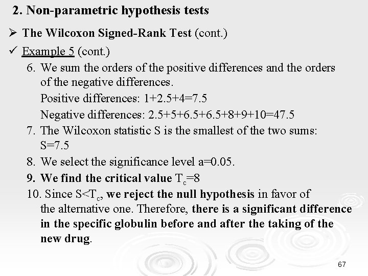
2. Non-parametric hypothesis tests Ø The Wilcoxon Signed-Rank Test (cont. ) ü Example 5 (cont. ) 6. We sum the orders of the positive differences and the orders of the negative differences. Positive differences: 1+2. 5+4=7. 5 Negative differences: 2. 5+5+6. 5+8+9+10=47. 5 7. The Wilcoxon statistic S is the smallest of the two sums: S=7. 5 8. We select the significance level a=0. 05. 9. We find the critical value Tc=8 10. Since S<Tc, we reject the null hypothesis in favor of the alternative one. Therefore, there is a significant difference in the specific globulin before and after the taking of the new drug. 67

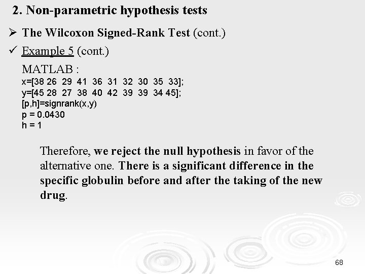
2. Non-parametric hypothesis tests Ø The Wilcoxon Signed-Rank Test (cont. ) ü Example 5 (cont. ) MATLAB : x=[38 26 29 41 36 31 32 30 35 33]; y=[45 28 27 38 40 42 39 39 34 45]; [p, h]=signrank(x, y) p = 0. 0430 h=1 Therefore, we reject the null hypothesis in favor of the alternative one. There is a significant difference in the specific globulin before and after the taking of the new drug. 68

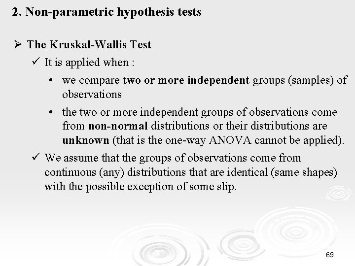
2. Non-parametric hypothesis tests Ø The Kruskal-Wallis Test ü It is applied when : • we compare two or more independent groups (samples) of observations • the two or more independent groups of observations come from non-normal distributions or their distributions are unknown (that is the one-way ANOVA cannot be applied). ü We assume that the groups of observations come from continuous (any) distributions that are identical (same shapes) with the possible exception of some slip. 69

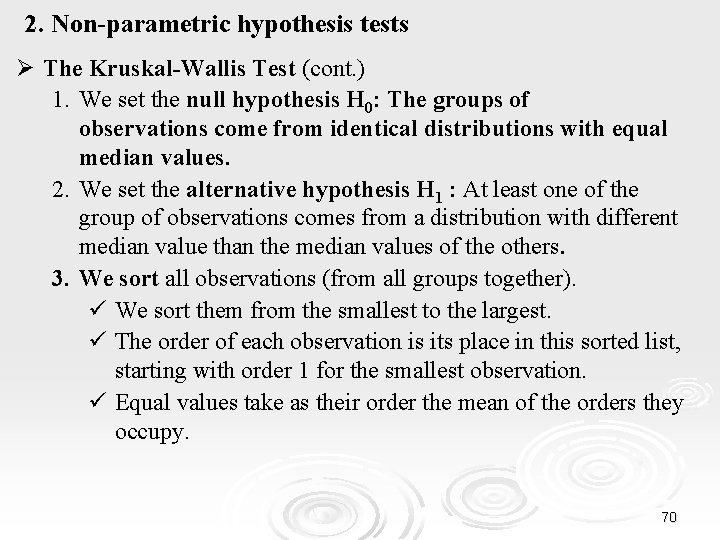
2. Non-parametric hypothesis tests Ø The Kruskal-Wallis Test (cont. ) 1. We set the null hypothesis H 0: The groups of observations come from identical distributions with equal median values. 2. We set the alternative hypothesis H 1 : At least one of the group of observations comes from a distribution with different median value than the median values of the others. 3. We sort all observations (from all groups together). ü We sort them from the smallest to the largest. ü The order of each observation is its place in this sorted list, starting with order 1 for the smallest observation. ü Equal values take as their order the mean of the orders they occupy. 70

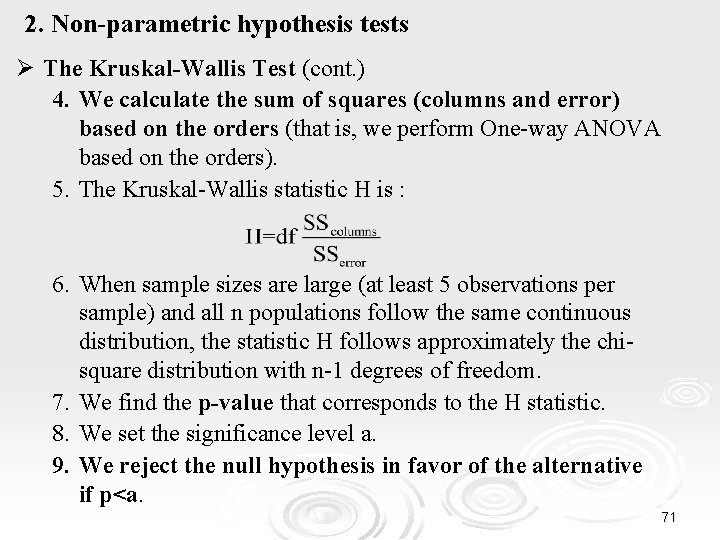
2. Non-parametric hypothesis tests Ø The Kruskal-Wallis Test (cont. ) 4. We calculate the sum of squares (columns and error) based on the orders (that is, we perform One-way ANOVA based on the orders). 5. The Kruskal-Wallis statistic H is : 6. When sample sizes are large (at least 5 observations per sample) and all n populations follow the same continuous distribution, the statistic H follows approximately the chisquare distribution with n-1 degrees of freedom. 7. We find the p-value that corresponds to the H statistic. 8. We set the significance level a. 9. We reject the null hypothesis in favor of the alternative if p<a. 71

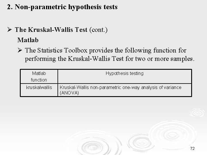
2. Non-parametric hypothesis tests Ø The Kruskal-Wallis Test (cont. ) Matlab Ø The Statistics Toolbox provides the following function for performing the Kruskal-Wallis Test for two or more samples. Matlab function kruskalwallis Hypothesis testing Kruskal-Wallis non-parametric one-way analysis of variance (ANOVA) 72

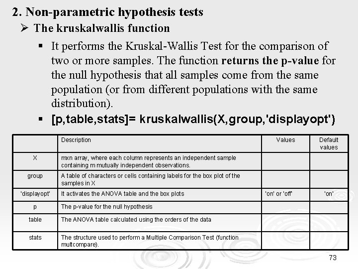
2. Non-parametric hypothesis tests Ø The kruskalwallis function § It performs the Kruskal-Wallis Test for the comparison of two or more samples. The function returns the p-value for the null hypothesis that all samples come from the same population (or from different populations with the same distribution). § [p, table, stats]= kruskalwallis(X, group, 'displayopt') Description X group ‘displayopt’ p Values Default values mxn array, where each column represents an independent sample containing m mutually independent observations. A table of characters or cells containing labels for the box plot of the samples in X It activates the ANOVA table and the box plots ‘on’ or ‘off’ ‘on’ The p-value for the null hypothesis table The ANOVA table calculated using the orders of the data stats The structure used to perform a Multiple Comparison Test (function multcompare). 73

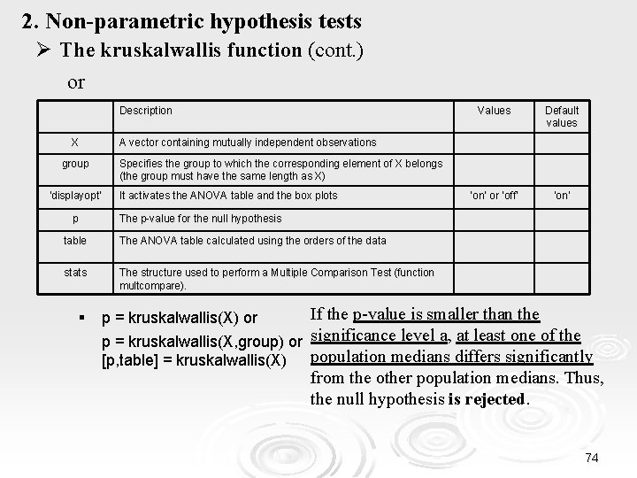
2. Non-parametric hypothesis tests Ø The kruskalwallis function (cont. ) or Description X ‘on’ or ‘off’ ‘on’ Specifies the group to which the corresponding element of X belongs (the group must have the same length as X) ‘displayopt’ It activates the ANOVA table and the box plots The p-value for the null hypothesis table The ANOVA table calculated using the orders of the data stats The structure used to perform a Multiple Comparison Test (function multcompare). § Default values A vector containing mutually independent observations group p Values If the p-value is smaller than the p = kruskalwallis(X, group) or significance level a, at least one of the population medians differs significantly [p, table] = kruskalwallis(X) from the other population medians. Thus, the null hypothesis is rejected. p = kruskalwallis(X) or 74

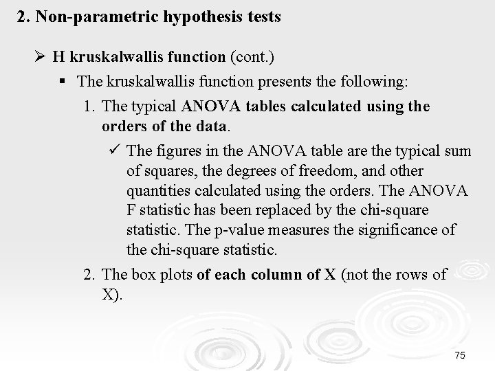
2. Non-parametric hypothesis tests Ø Η kruskalwallis function (cont. ) § The kruskalwallis function presents the following: 1. The typical ANOVA tables calculated using the orders of the data. ü The figures in the ANOVA table are the typical sum of squares, the degrees of freedom, and other quantities calculated using the orders. The ANOVA F statistic has been replaced by the chi-square statistic. The p-value measures the significance of the chi-square statistic. 2. The box plots of each column of X (not the rows of X). 75

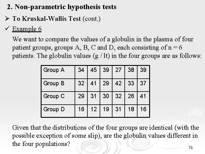
2. Non-parametric hypothesis tests Ø Το Kruskal-Wallis Test (cont. ) ü Example 6 We want to compare the values of a globulin in the plasma of four patient groups, groups A, B, C and D, each consisting of n = 6 patients. The globulin values (g / lt) in the four groups are as follows: Group A 34 45 39 27 38 39 Group B 32 41 29 42 33 37 Group C 29 31 30 32 26 41 Group D 16 12 19 31 18 16 Given that the distributions of the four groups are identical (with the possible exception of some slip), are the globulin values different in the four populations? 76

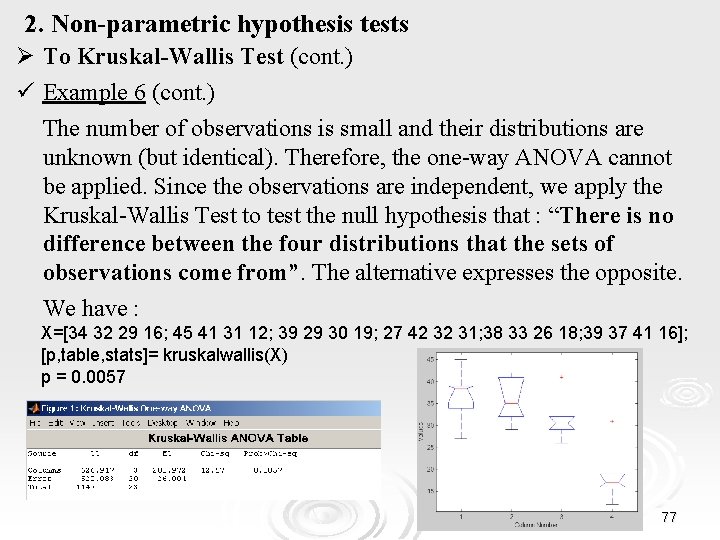
2. Non-parametric hypothesis tests Ø Το Kruskal-Wallis Test (cont. ) ü Example 6 (cont. ) The number of observations is small and their distributions are unknown (but identical). Therefore, the one-way ANOVA cannot be applied. Since the observations are independent, we apply the Kruskal-Wallis Test to test the null hypothesis that : “There is no difference between the four distributions that the sets of observations come from”. The alternative expresses the opposite. We have : X=[34 32 29 16; 45 41 31 12; 39 29 30 19; 27 42 32 31; 38 33 26 18; 39 37 41 16]; [p, table, stats]= kruskalwallis(X) p = 0. 0057 77

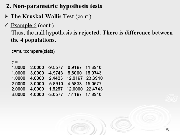
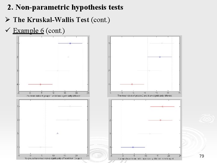
2. Non-parametric hypothesis tests Ø The Kruskal-Wallis Test (cont. ) ü Example 6 (cont. ) Thus, the null hypothesis is rejected. There is difference between the 4 populations. c=multcompare(stats) c= 1. 0000 2. 0000 3. 0000 4. 0000 -9. 5577 0. 9167 11. 3910 -4. 9743 5. 5000 15. 9743 2. 4423 12. 9167 23. 3910 -5. 8910 4. 5833 15. 0577 1. 5257 12. 0000 22. 4743 -3. 0577 7. 4167 17. 8910 78

2. Non-parametric hypothesis tests Ø The Kruskal-Wallis Test (cont. ) ü Example 6 (cont. ) 79

Examples for hypothesis tests for normality and chi-square 2. Non-parametric hypothesis tests 3. Selection of the statistical test 1. 80

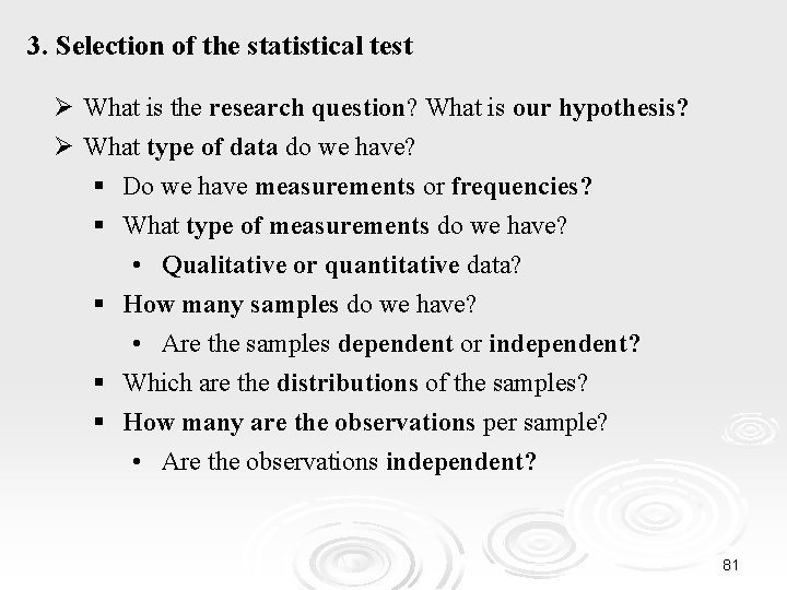
3. Selection of the statistical test Ø What is the research question? What is our hypothesis? Ø What type of data do we have? § Do we have measurements or frequencies? § What type of measurements do we have? • Qualitative or quantitative data? § How many samples do we have? • Are the samples dependent or independent? § Which are the distributions of the samples? § How many are the observations per sample? • Are the observations independent? 81

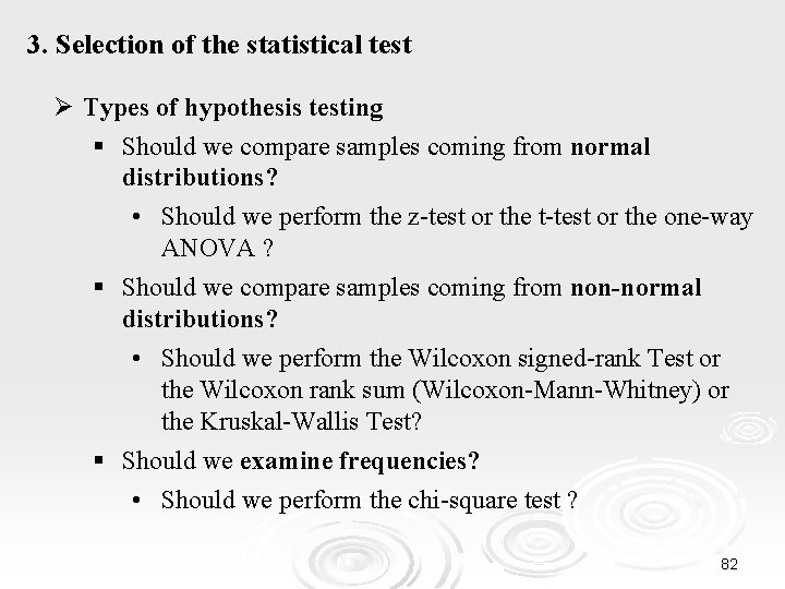
3. Selection of the statistical test Ø Types of hypothesis testing § Should we compare samples coming from normal distributions? • Should we perform the z-test or the t-test or the one-way ANOVA ? § Should we compare samples coming from non-normal distributions? • Should we perform the Wilcoxon signed-rank Test or the Wilcoxon rank sum (Wilcoxon-Mann-Whitney) or the Kruskal-Wallis Test? § Should we examine frequencies? • Should we perform the chi-square test ? 82

3. Selection of the statistical test Ø Having chosen the hypothesis test, we must consider the following questions : § Which hypotheses are being tested? § What conditions must be fulfilled? § Which diagrams are useful? § What alternatives are available if conditions are not fulfilled? § What is the test statistic? § What are the degrees of freedom? 83