MULTIPLE TESTING POWER AND TYPE I ERROR Andrew

MULTIPLE TESTING: POWER AND TYPE I ERROR Andrew Morris Wellcome Trust Centre for Human Genetics March 7, 2003

Outline Multiple testing. ¡ Bonferonni correction. ¡ Genome-wide association studies. ¡ Randomisation procedures. ¡ LOD scores and genome-wide significance levels for linkage. ¡

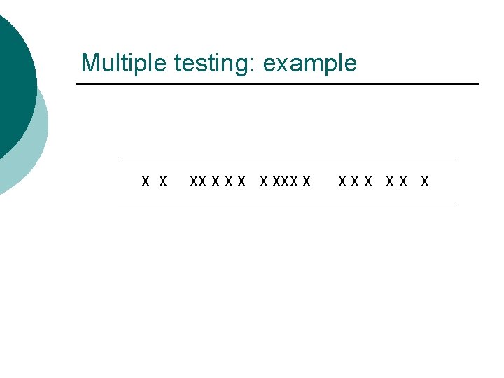
Multiple testing: example X X XXX XX X

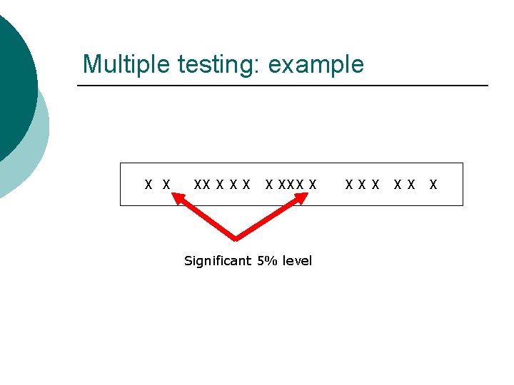
Multiple testing: example X X XXX X Significant 5% level XXX XX X

Multiple testing ¡ ¡ Significance level α. Perform N independent tests of null hypothesis. Number of tests in which null hypothesis is rejected, in samples ascertained from population in which null hypothesis is true, given by binomial distribution, parameters N and α. Expect to see Nα rejections of null hypothesis by chance.

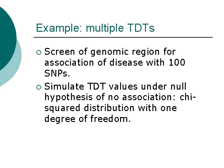
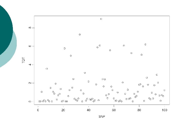
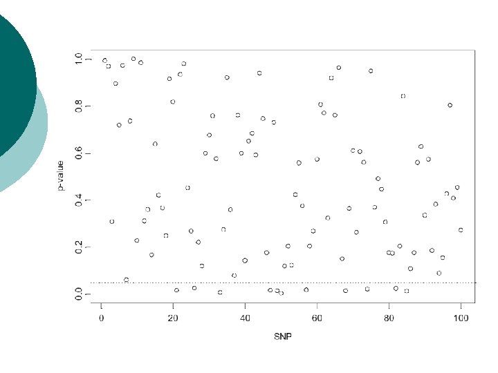
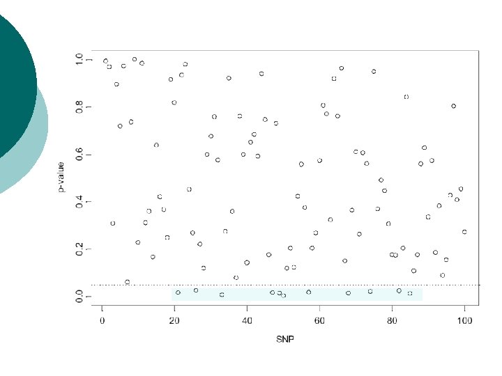
Example: multiple TDTs Screen of genomic region for association of disease with 100 SNPs. ¡ Simulate TDT values under null hypothesis of no association: chisquared distribution with one degree of freedom. ¡

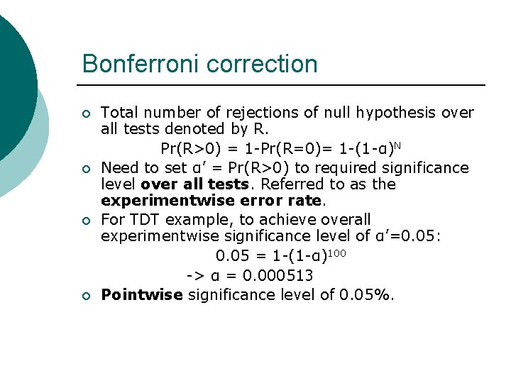
Bonferroni correction ¡ ¡ Total number of rejections of null hypothesis over all tests denoted by R. Pr(R>0) = 1 -Pr(R=0)= 1 -(1 -α)N Need to set α’ = Pr(R>0) to required significance level over all tests. Referred to as the experimentwise error rate. For TDT example, to achieve overall experimentwise significance level of α’=0. 05: 0. 05 = 1 -(1 -α)100 -> α = 0. 000513 Pointwise significance level of 0. 05%.

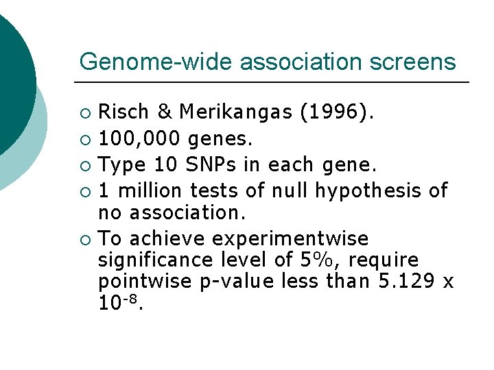
Genome-wide association screens Risch & Merikangas (1996). ¡ 100, 000 genes. ¡ Type 10 SNPs in each gene. ¡ 1 million tests of null hypothesis of no association. ¡ To achieve experimentwise significance level of 5%, require pointwise p-value less than 5. 129 x 10 -8. ¡

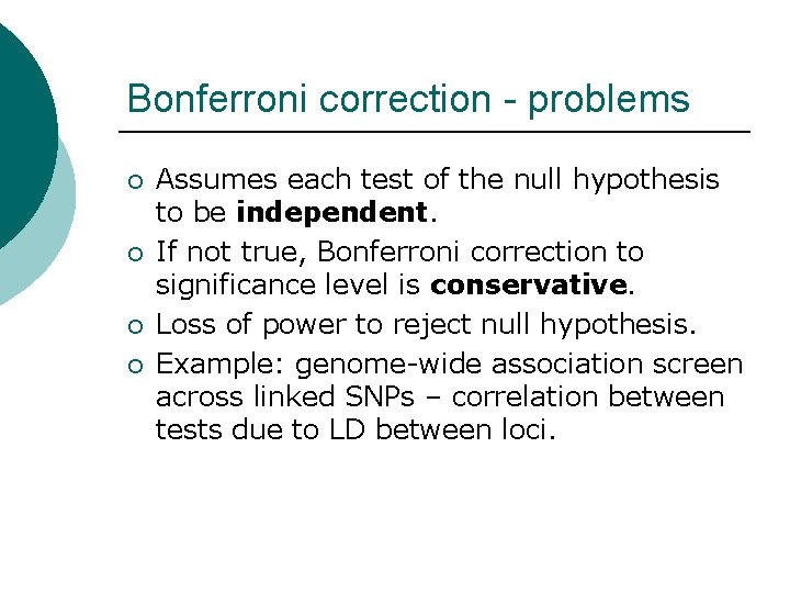
Bonferroni correction - problems ¡ ¡ Assumes each test of the null hypothesis to be independent. If not true, Bonferroni correction to significance level is conservative. Loss of power to reject null hypothesis. Example: genome-wide association screen across linked SNPs – correlation between tests due to LD between loci.

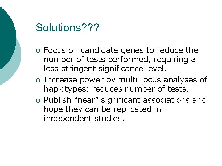
Solutions? ? ? ¡ ¡ ¡ Focus on candidate genes to reduce the number of tests performed, requiring a less stringent significance level. Increase power by multi-locus analyses of haplotypes: reduces number of tests. Publish “near” significant associations and hope they can be replicated in independent studies.

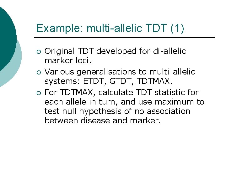
Example: multi-allelic TDT (1) ¡ ¡ ¡ Original TDT developed for di-allelic marker loci. Various generalisations to multi-allelic systems: ETDT, GTDT, TDTMAX. For TDTMAX, calculate TDT statistic for each allele in turn, and use maximum to test null hypothesis of no association between disease and marker.

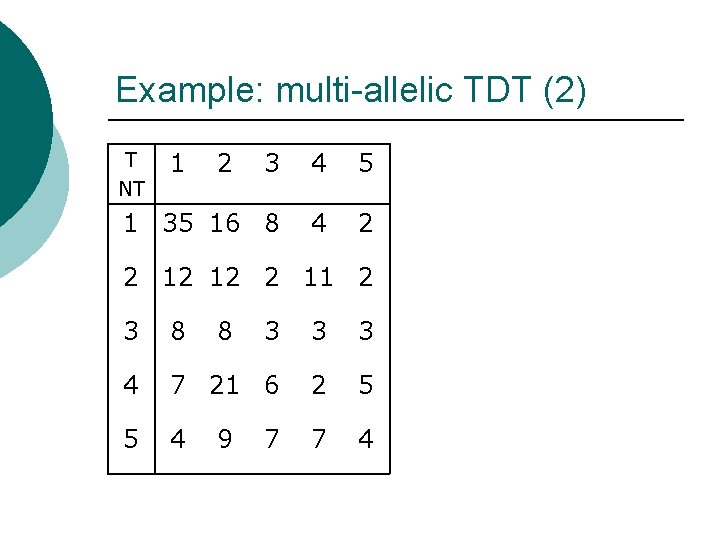
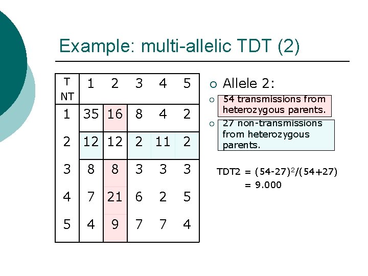
Example: multi-allelic TDT (2) 3 4 5 1 35 16 8 4 2 T NT 1 2 2 12 12 2 11 2 3 8 8 3 3 3 4 7 21 6 2 5 5 4 7 4 9 7

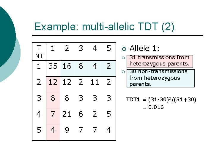
Example: multi-allelic TDT (2) T NT 1 2 3 4 5 ¡ ¡ 1 35 16 8 4 2 2 12 12 2 11 2 3 8 8 3 3 3 4 7 21 6 2 5 5 4 7 4 9 7 ¡ Allele 1: 31 transmissions from heterozygous parents. 30 non-transmissions from heterozygous parents. TDT 1 = (31 -30)2/(31+30) = 0. 016

Example: multi-allelic TDT (2) T NT 1 2 3 4 5 ¡ ¡ 1 35 16 8 4 2 2 12 12 2 11 2 3 8 8 3 3 3 4 7 21 6 2 5 5 4 7 4 9 7 ¡ Allele 2: 54 transmissions from heterozygous parents. 27 non-transmissions from heterozygous parents. TDT 2 = (54 -27)2/(54+27) = 9. 000

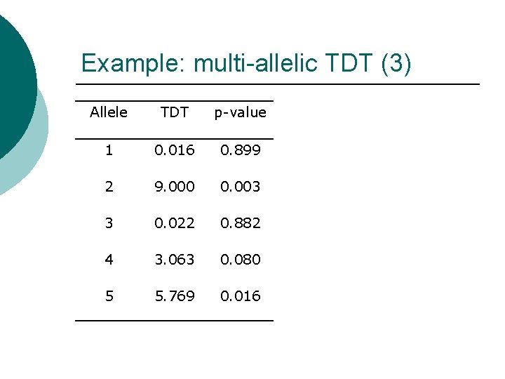
Example: multi-allelic TDT (3) Allele TDT p-value 1 0. 016 0. 899 2 9. 000 0. 003 3 0. 022 0. 882 4 3. 063 0. 080 5 5. 769 0. 016

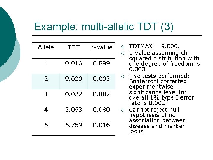
Example: multi-allelic TDT (3) Allele TDT p-value ¡ ¡ 1 0. 016 0. 899 2 9. 000 0. 003 3 0. 022 0. 882 4 3. 063 0. 080 5 5. 769 0. 016 ¡ ¡ TDTMAX = 9. 000. p-value assuming chisquared distribution with one degree of freedom is 0. 003. Five tests performed: Bonferroni corrected experimentwise significance level for overall 1% type I error rate is 0. 002. Cannot reject null hypothesis of no association between disease and marker locus.

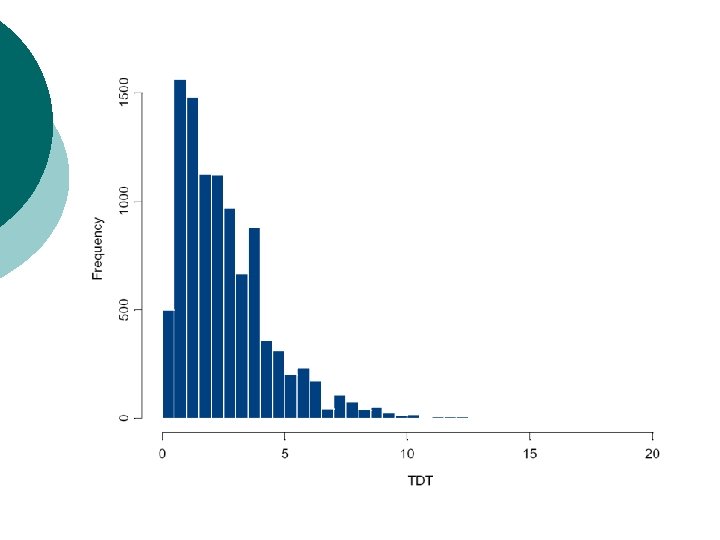
Example: multi-allelic TDT (4) Bonferonni correction conservative since TDTs for multiple alleles at same locus are correlated. ¡ Generate null distribution of TDTMAX statistic by simulation. ¡ Randomisation procedures… ¡

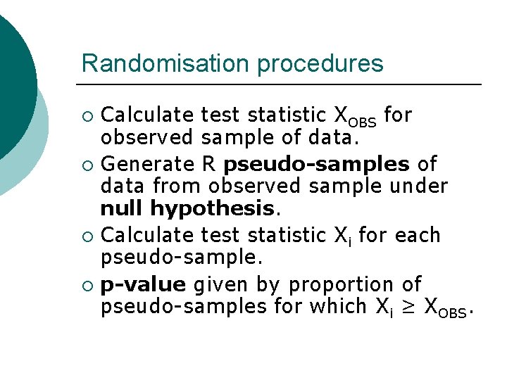
Randomisation procedures Calculate test statistic XOBS for observed sample of data. ¡ Generate R pseudo-samples of data from observed sample under null hypothesis. ¡ Calculate test statistic Xi for each pseudo-sample. ¡ p-value given by proportion of pseudo-samples for which Xi ≥ XOBS. ¡

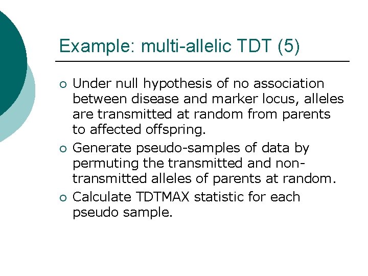
Example: multi-allelic TDT (5) ¡ ¡ ¡ Under null hypothesis of no association between disease and marker locus, alleles are transmitted at random from parents to affected offspring. Generate pseudo-samples of data by permuting the transmitted and nontransmitted alleles of parents at random. Calculate TDTMAX statistic for each pseudo sample.

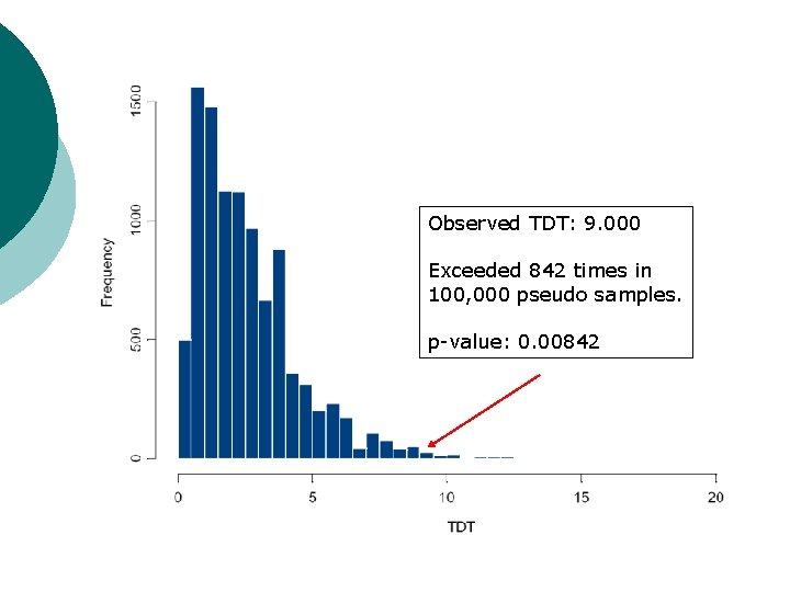
Observed TDT: 9. 000 Exceeded 842 times in 100, 000 pseudo samples. p-value: 0. 00842

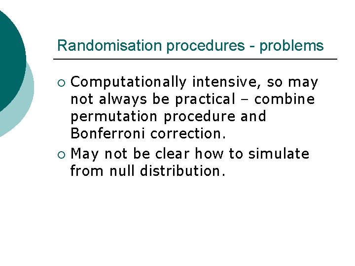
Randomisation procedures - problems Computationally intensive, so may not always be practical – combine permutation procedure and Bonferroni correction. ¡ May not be clear how to simulate from null distribution. ¡

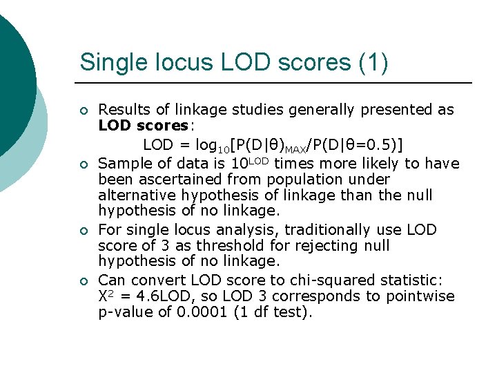
Single locus LOD scores (1) ¡ ¡ Results of linkage studies generally presented as LOD scores: LOD = log 10[P(D|θ)MAX/P(D|θ=0. 5)] Sample of data is 10 LOD times more likely to have been ascertained from population under alternative hypothesis of linkage than the null hypothesis of no linkage. For single locus analysis, traditionally use LOD score of 3 as threshold for rejecting null hypothesis of no linkage. Can convert LOD score to chi-squared statistic: X 2 = 4. 6 LOD, so LOD 3 corresponds to pointwise p-value of 0. 0001 (1 df test).

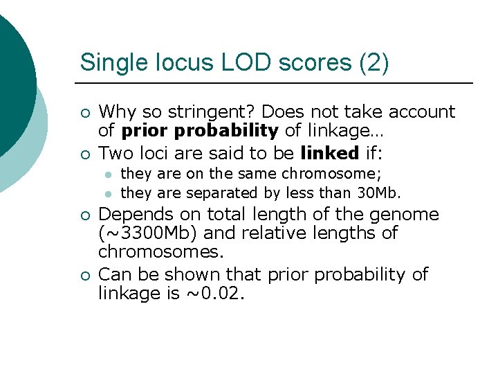
Single locus LOD scores (2) ¡ ¡ Why so stringent? Does not take account of prior probability of linkage… Two loci are said to be linked if: l l ¡ ¡ they are on the same chromosome; they are separated by less than 30 Mb. Depends on total length of the genome (~3300 Mb) and relative lengths of chromosomes. Can be shown that prior probability of linkage is ~0. 02.

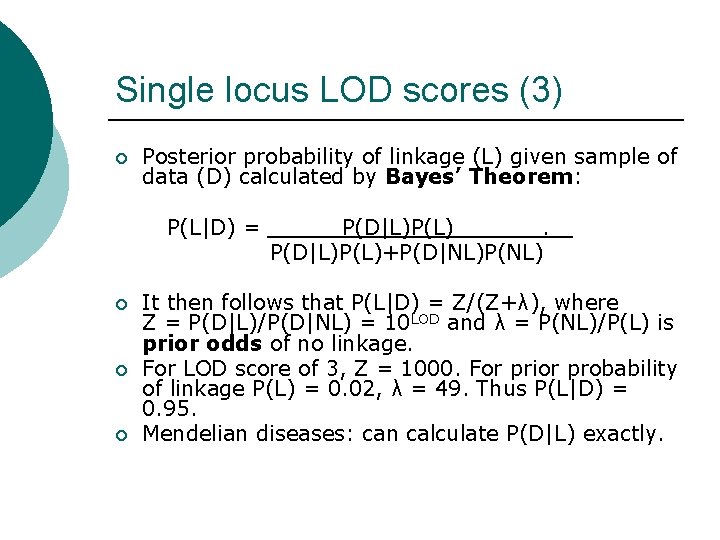
Single locus LOD scores (3) ¡ Posterior probability of linkage (L) given sample of data (D) calculated by Bayes’ Theorem: P(L|D) = ¡ ¡ ¡ P(D|L)P(L)+P(D|NL)P(NL) It then follows that P(L|D) = Z/(Z+λ), where Z = P(D|L)/P(D|NL) = 10 LOD and λ = P(NL)/P(L) is prior odds of no linkage. For LOD score of 3, Z = 1000. For prior probability of linkage P(L) = 0. 02, λ = 49. Thus P(L|D) = 0. 95. Mendelian diseases: can calculate P(D|L) exactly.

LOD scores: genome screen ¡ ¡ ¡ Search of the genome for evidence of linkage using multiple markers. Could adjust significance level by Bonferroni correction, but does not take account of the strong correlation between linked markers. Lander & Kruglyak (1995) propose calculation of genome-wide significance level to allow for multiple testing.

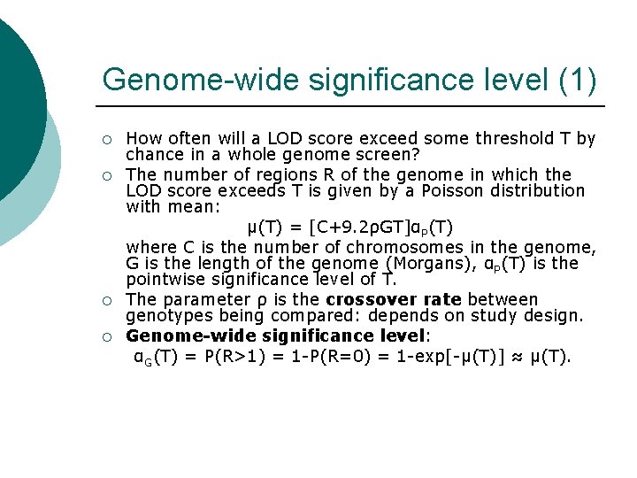
Genome-wide significance level (1) ¡ ¡ How often will a LOD score exceed some threshold T by chance in a whole genome screen? The number of regions R of the genome in which the LOD score exceeds T is given by a Poisson distribution with mean: μ(T) = [C+9. 2ρGT]αP(T) where C is the number of chromosomes in the genome, G is the length of the genome (Morgans), αP(T) is the pointwise significance level of T. The parameter ρ is the crossover rate between genotypes being compared: depends on study design. Genome-wide significance level: αG(T) = P(R>1) = 1 -P(R=0) = 1 -exp[-μ(T)] ≈ μ(T).

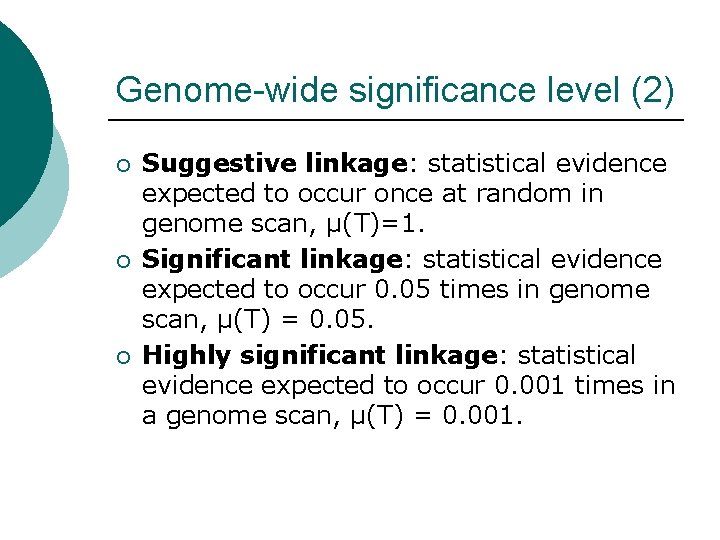
Genome-wide significance level (2) ¡ ¡ ¡ Suggestive linkage: statistical evidence expected to occur once at random in genome scan, μ(T)=1. Significant linkage: statistical evidence expected to occur 0. 05 times in genome scan, μ(T) = 0. 05. Highly significant linkage: statistical evidence expected to occur 0. 001 times in a genome scan, μ(T) = 0. 001.

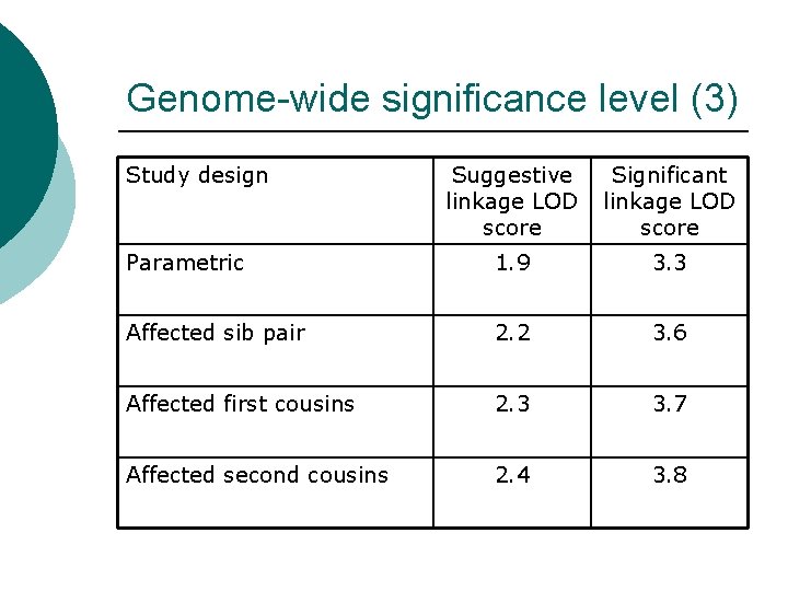
Genome-wide significance level (3) Study design Suggestive linkage LOD score Significant linkage LOD score Parametric 1. 9 3. 3 Affected sib pair 2. 2 3. 6 Affected first cousins 2. 3 3. 7 Affected second cousins 2. 4 3. 8

Genome-wide significance level (4) ¡ Is the genome-wide significance level too stringent: l l Study only looked at a few markers? NO: likely that study stopped after first significant linkage – investigator may have continued until entire genome searched if no positive signals identified. Study involved sparse screen of genome? NO: likely that positive signals will be followed up by higher density searches.

Examples ¡ IDDM l l l ¡ 96 sib pairs: average 10 c. M spacing. Followed up regions with LOD > 1, with additional sib pair sets. Significant linkage at HLA, suggestive linkage on 8 q and X, near suggestive linkages on 11 q and 6 q. Schizophrenia l l Near significant linkages on chromosome 6 p in large collection of pedigrees. Replicated in two independent data sets.

Replication ¡ ¡ ¡ Linkage and association signals must be replicated in independent studies to be credible. Replication studies test an established prior hypothesis, so multiple testing problem not an issue. Failure to replicate does not disprove the linkage or association, unless the power of the replication study is very high. Competing results of several replication studies may reflect population heterogeneity, diagnostic differences, random sample variation. Combined analysis or meta analysis…

Summary Multiple testing inflates the type I error rate of hypothesis test. ¡ Need stringent significance levels. ¡ Bonferroni correction conservative. ¡ Guidelines are available for genomewide linkage studies. ¡ Replication of results necessary for confirmation. ¡