Lecture 7 Smart Scheduling and Dispatching Policies Thrasyvoulos

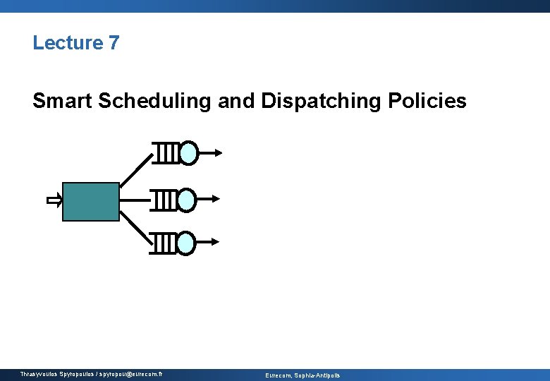
Lecture 7 Smart Scheduling and Dispatching Policies Thrasyvoulos Spyropoulos / spyropou@eurecom. fr Eurecom, Sophia-Antipolis

Single Server Model (M/G/1) Load r = l. E[X]<1 Poisson arrival process w/rate l X: job size (service requirement) Bounded Pareto Job sizes with huge variance are everywhere in CS: 1 • CPU Lifetimes of UNIX jobs [Harchol-Balter, Downey 96] • Supercomputing job sizes [Schroeder, Harchol-Balter 00] • Web file sizes [Crovella, Bestavros 98, Barford, Crovella 98] ½ Huge • IP Flow durations [Shaikh, Rexford, Shin 99] D. F. R. Variability ¼ Top-heavy: top 1% jobs make up half load Thrasyvoulos Spyropoulos / spyropou@eurecom. fr Eurecom, Sophia-Antipolis

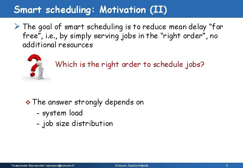
Outline Ø Smart scheduling Performance metrics v Policies classification v Examples v Ladies first! + they’ll go out first Ø Scheduling policies comparison (Fairness, Latency) Ø Task assignment problem Supercomputing and web server models v Optimal dispatching/scheduling policies v Thrasyvoulos Spyropoulos / spyropou@eurecom. fr Eurecom, Sophia-Antipolis 3

Smart scheduling: Motivation (I) Ø Why scheduling matters? Why doesn’t it work? ! ! Bla, bla… Why doesn’t it work? ! Bla, bla… !! Delay due to other users who are currently sharing the service !! Thrasyvoulos Spyropoulos / spyropou@eurecom. fr Eurecom, Sophia-Antipolis 4

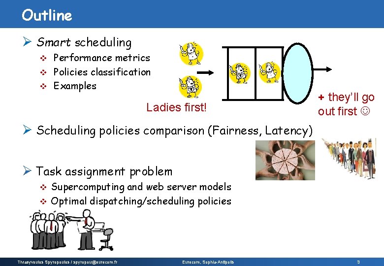
Smart scheduling: Motivation (II) Ø The goal of smart scheduling is to reduce mean delay “for free”, i. e. , by simply serving jobs in the “right order”, no additional resources Which is the right order to schedule jobs? v The answer strongly depends on - system load - job size distribution Thrasyvoulos Spyropoulos / spyropou@eurecom. fr Eurecom, Sophia-Antipolis 5

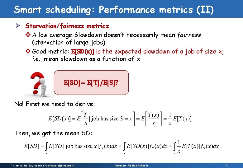
Smart scheduling: Performance metrics (I) Ø Common metrics to compare scheduling policies v E[T], mean response time v E[N], mean number (of jobs) in system v E[TQ], mean waiting time (= E[T]-E[S], where E[S]=service time) v Slowdown: SD=T/S (response time normalized by the running time) - Meaning: if a job takes twice as long to run due to system load, it suffers from a Slowdown factor of 2, etc. - Job response time should be proportional to its running time. Ideally: • small jobs → small response times • big jobs → big response times Thrasyvoulos Spyropoulos / spyropou@eurecom. fr Eurecom, Sophia-Antipolis 6

Smart scheduling: Performance metrics (II) Ø Starvation/fairness metrics v A low average Slowdown doesn’t necessarily mean fairness (starvation of large jobs) v Good metric: E[SD(x)] is the expected slowdown of a job of size x, i. e. , mean slowdown as a function of x E[SD]= E[T]/E[S]? No! First we need to derive: Then, we get the mean SD: Thrasyvoulos Spyropoulos / spyropou@eurecom. fr Eurecom, Sophia-Antipolis 7

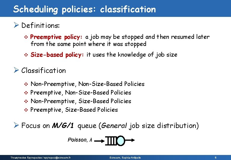
Scheduling policies: classification Ø Definitions: v Preemptive policy: a job may be stopped and then resumed later from the same point where it was stopped v Size-based policy: it uses the knowledge of job size Ø Classification Non-Preemptive, Non-Size-Based Policies v Non-Preemptive, Size-Based Policies v Ø Focus on M/G/1 queue (General job size distribution) Poisson, λ Thrasyvoulos Spyropoulos / spyropou@eurecom. fr Eurecom, Sophia-Antipolis 8

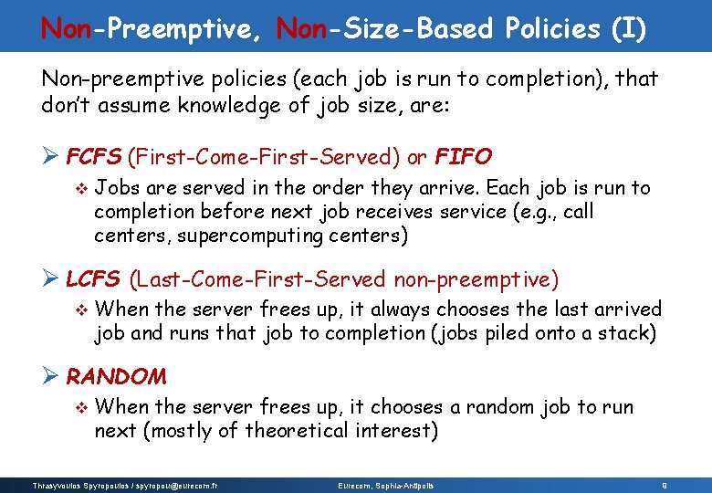
Non-Preemptive, Non-Size-Based Policies (I) Non-preemptive policies (each job is run to completion), that don’t assume knowledge of job size, are: Ø FCFS (First-Come-First-Served) or FIFO v Jobs are served in the order they arrive. Each job is run to completion before next job receives service (e. g. , call centers, supercomputing centers) Ø LCFS (Last-Come-First-Served non-preemptive) v When the server frees up, it always chooses the last arrived job and runs that job to completion (jobs piled onto a stack) Ø RANDOM v When the server frees up, it chooses a random job to run next (mostly of theoretical interest) Thrasyvoulos Spyropoulos / spyropou@eurecom. fr Eurecom, Sophia-Antipolis 9

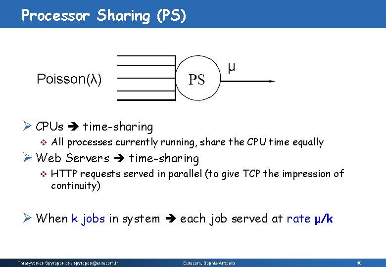
Processor Sharing (PS) μ Poisson(λ) Ø CPUs time-sharing v All processes currently running, share the CPU time equally Ø Web Servers time-sharing v HTTP requests served in parallel (to give TCP the impression of continuity) Ø When k jobs in system each job served at rate μ/k Thrasyvoulos Spyropoulos / spyropou@eurecom. fr Eurecom, Sophia-Antipolis 10

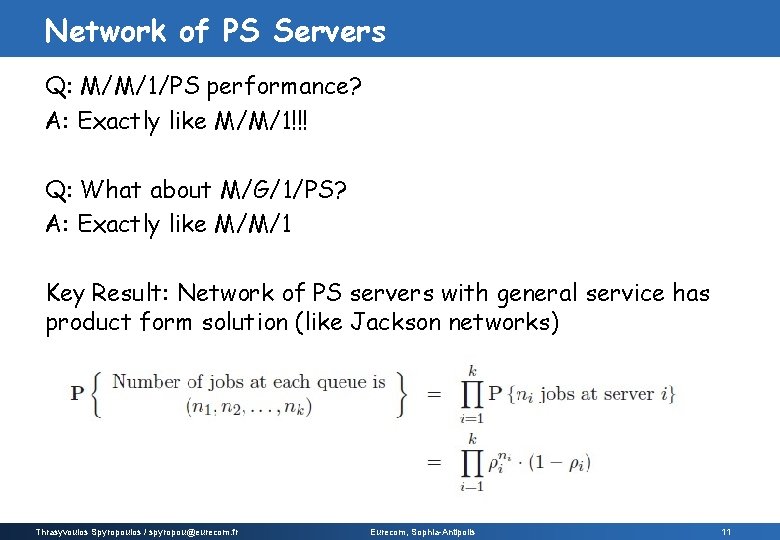
Network of PS Servers Q: M/M/1/PS performance? A: Exactly like M/M/1!!! Q: What about M/G/1/PS? A: Exactly like M/M/1 Key Result: Network of PS servers with general service has product form solution (like Jackson networks) Thrasyvoulos Spyropoulos / spyropou@eurecom. fr Eurecom, Sophia-Antipolis 11

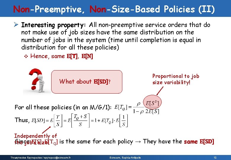
Non-Preemptive, Non-Size-Based Policies (II) Ø Interesting property: All non-preemptive service orders that do not make use of job sizes have the same distribution on the number of jobs in the system (time until completion is equal in distribution for all these policies) v Hence, same E[T], E[N] What about E[SD]? Proportional to job size variability! For all these policies (in an M/G/1): Thus, Independently of Since E[S], E[TQ] is the same for each policy → They have the same E[SD] the job’s size! Thrasyvoulos Spyropoulos / spyropou@eurecom. fr Eurecom, Sophia-Antipolis 12

Preemptive, Non-Size-Based Policies (I) Ø So far: non-preemptive/non-size-based service E[T] can be very high when job size variability is high v Intuition: short jobs queue up behind long jobs v Ø Processor-Sharing (PS): when a job arrives, it immediately shares the capacity with all the current jobs (Ex. R. R. CPU scheduling) + PS allows short jobs to get out quickly, helps to reduce E[T], E[SD] (compared to FCFS), increases system throughput (different jobs run simultaneously) - PS is not better than FCFS on every arrival sequence + Mean response time for PS is insensitive to job size variability: E[T]M/G/1/PS= E[S] / (1 -ρ) where ρ is the system utilization (load) Thrasyvoulos Spyropoulos / spyropou@eurecom. fr Eurecom, Sophia-Antipolis 13

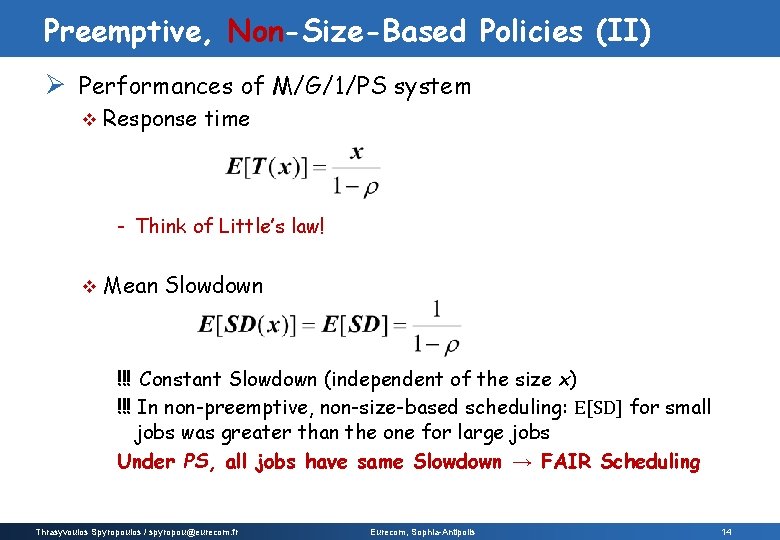
Preemptive, Non-Size-Based Policies (II) Ø Performances of M/G/1/PS system v Response time - Think of Little’s law! v Mean Slowdown !!! Constant Slowdown (independent of the size x) !!! In non-preemptive, non-size-based scheduling: E[SD] for small jobs was greater than the one for large jobs Under PS, all jobs have same Slowdown → FAIR Scheduling Thrasyvoulos Spyropoulos / spyropou@eurecom. fr Eurecom, Sophia-Antipolis 14

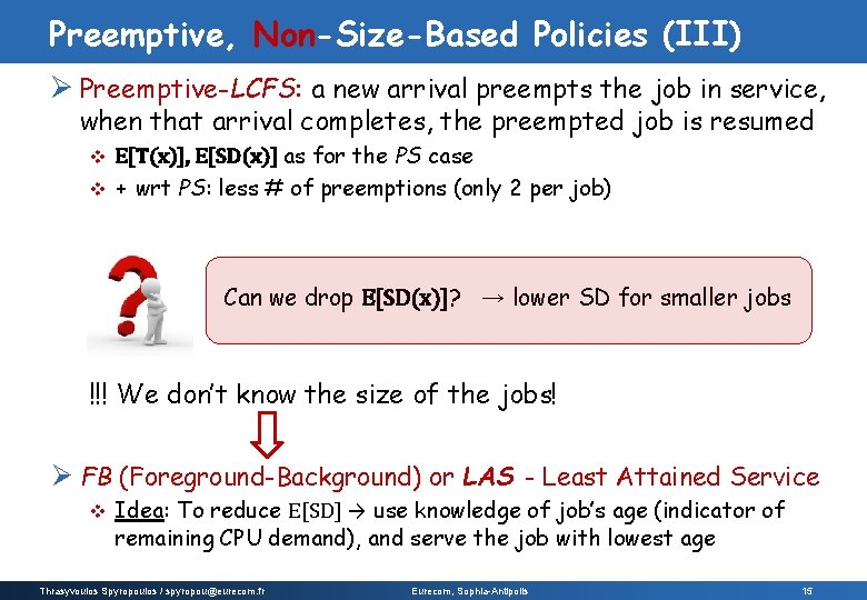
Preemptive, Non-Size-Based Policies (III) Ø Preemptive-LCFS: a new arrival preempts the job in service, when that arrival completes, the preempted job is resumed E[T(x)], E[SD(x)] as for the PS case v + wrt PS: less # of preemptions (only 2 per job) v Can we drop E[SD(x)]? → lower SD for smaller jobs !!! We don’t know the size of the jobs! Ø FB (Foreground-Background) or LAS - Least Attained Service v Idea: To reduce E[SD] → use knowledge of job’s age (indicator of remaining CPU demand), and serve the job with lowest age Thrasyvoulos Spyropoulos / spyropou@eurecom. fr Eurecom, Sophia-Antipolis 15

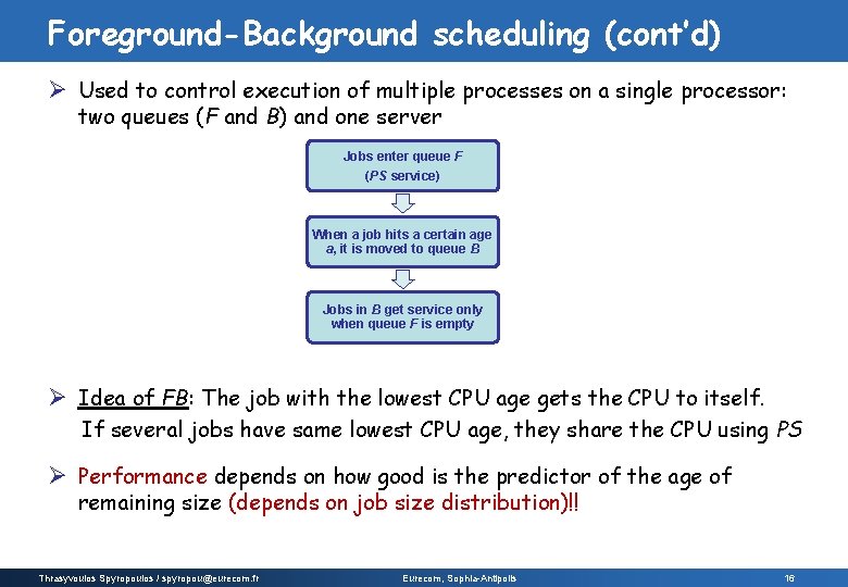
Foreground-Background scheduling (cont’d) Ø Used to control execution of multiple processes on a single processor: two queues (F and B) and one server Jobs enter queue F (PS service) When a job hits a certain age a, it is moved to queue B Jobs in B get service only when queue F is empty Ø Idea of FB: The job with the lowest CPU age gets the CPU to itself. If several jobs have same lowest CPU age, they share the CPU using PS Ø Performance depends on how good is the predictor of the age of remaining size (depends on job size distribution)!! Thrasyvoulos Spyropoulos / spyropou@eurecom. fr Eurecom, Sophia-Antipolis 16

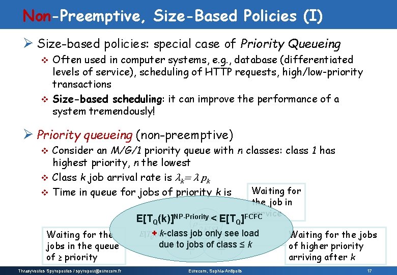
Non-Preemptive, Size-Based Policies (I) Ø Size-based policies: special case of Priority Queueing Often used in computer systems, e. g. , database (differentiated levels of service), scheduling of HTTP requests, high/low-priority transactions v Size-based scheduling: it can improve the performance of a system tremendously! v Ø Priority queueing (non-preemptive) Consider an M/G/1 priority queue with n classes: class 1 has highest priority, n the lowest v Class k job arrival rate is λk= λ pk Waiting for v Time in queue for jobs of priority k is v E[TQ(k)]NP-Priority < E[TQ] Waiting for the jobs in the queue of ≥ priority Thrasyvoulos Spyropoulos / spyropou@eurecom. fr the job in service FCFC + k-class job only see load due to jobs of class ≤ k Eurecom, Sophia-Antipolis Waiting for the jobs of higher priority arriving after k 17

Non-Preemptive, Size-Based Policies (II) Ø Question: If you want to minimize E[T], who should have higher priority: large or small jobs? Ø Theorem: Consider an NP-Priority M/G/1 with two classes of jobs: small (S) and large (L). To minimize E[T], class S jobs should have priority over class L jobs (since E[SS]<E[SL]) Ø SJF - Non-preemptive Shortest Job First v Whenever the server is free, it chooses the job with the smallest size (once a job is running, it is never interrupted) - Under heavy-tailed distributions, E[TQ] is smaller than the FCFS one (since most jobs are small) - But, mean delay is proportional to the variance → large delays for very high variance - Small jobs can still get stuck behind a big one (already running) → need of preemption! Thrasyvoulos Spyropoulos / spyropou@eurecom. fr Eurecom, Sophia-Antipolis 18

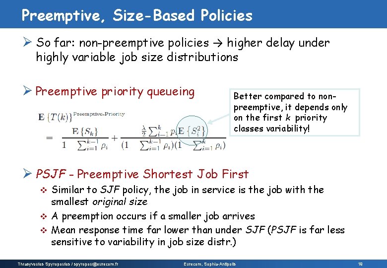
Preemptive, Size-Based Policies Ø So far: non-preemptive policies → higher delay under highly variable job size distributions Ø Preemptive priority queueing Better compared to nonpreemptive, it depends only on the first k priority classes variability! Ø PSJF - Preemptive Shortest Job First Similar to SJF policy, the job in service is the job with the smallest original size v A preemption occurs if a smaller job arrives v Mean response time far lower than under SJF (PSJF is far less sensitive to variability in job size distr. ) v Thrasyvoulos Spyropoulos / spyropou@eurecom. fr Eurecom, Sophia-Antipolis 19

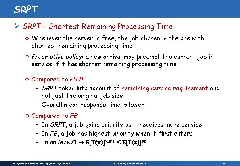
SRPT Ø SRPT - Shortest Remaining Processing Time v Whenever the server is free, the job chosen is the one with shortest remaining processing time v Preemptive policy: a new arrival may preempt the current job in service if it has shorter remaining processing time v Compared to PSJF - SRPT takes into account of remaining service requirement and not just the original job size - Overall mean response time is lower v Compared to FB - In SRPT, a job gains priority as it receives more service - In FB, a job has highest priority when it first enters - In an M/G/1 → E[T(x)]SRPT ≤ E[T(x)]FB Thrasyvoulos Spyropoulos / spyropou@eurecom. fr Eurecom, Sophia-Antipolis 20

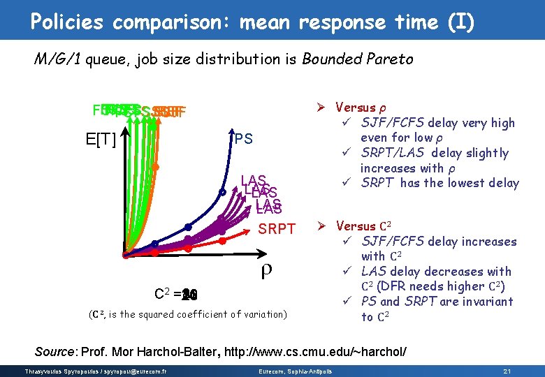
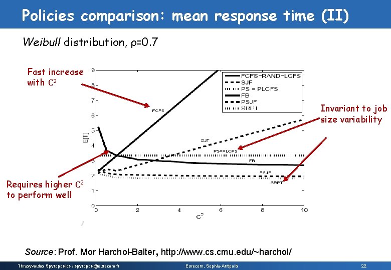
Policies comparison: mean response time (I) M/G/1 queue, job size distribution is Bounded Pareto FCFS SJF SJF FCFS SJF E[T] PS LAS LAS LAS SRPT r C 2 =24 8 16 12 20 (C 2, is the squared coefficient of variation) Ø Versus ρ ü SJF/FCFS delay very high even for low ρ ü SRPT/LAS delay slightly increases with ρ ü SRPT has the lowest delay Ø Versus C 2 ü SJF/FCFS delay increases with C 2 ü LAS delay decreases with C 2 (DFR needs higher C 2) ü PS and SRPT are invariant to C 2 Source: Prof. Mor Harchol-Balter, http: //www. cs. cmu. edu/~harchol/ Thrasyvoulos Spyropoulos / spyropou@eurecom. fr Eurecom, Sophia-Antipolis 21

Policies comparison: mean response time (II) Weibull distribution, ρ=0. 7 Fast increase with C 2 Invariant to job size variability Requires higher C 2 to perform well Source: Prof. Mor Harchol-Balter, http: //www. cs. cmu. edu/~harchol/ Thrasyvoulos Spyropoulos / spyropou@eurecom. fr Eurecom, Sophia-Antipolis 22

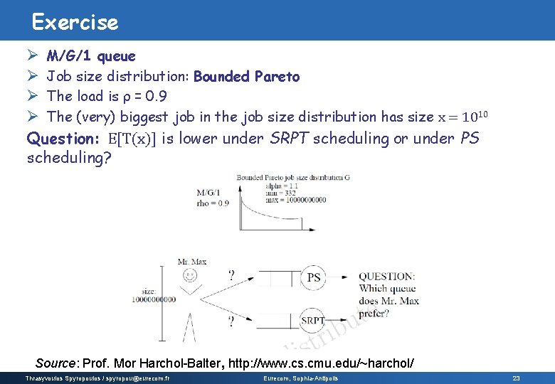
Exercise Ø M/G/1 queue Ø Job size distribution: Bounded Pareto Ø The load is ρ = 0. 9 Ø The (very) biggest job in the job size distribution has size x = 1010 Question: E[T(x)] is lower under SRPT scheduling or under PS scheduling? Source: Prof. Mor Harchol-Balter, http: //www. cs. cmu. edu/~harchol/ Thrasyvoulos Spyropoulos / spyropou@eurecom. fr Eurecom, Sophia-Antipolis 23

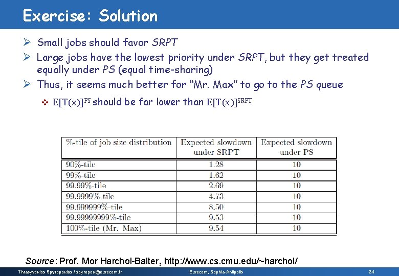
Exercise: Solution Ø Small jobs should favor SRPT Ø Large jobs have the lowest priority under SRPT, but they get treated equally under PS (equal time-sharing) Ø Thus, it seems much better for “Mr. Max” to go to the PS queue v E[T(x)]PS should be far lower than E[T(x)]SRPT Source: Prof. Mor Harchol-Balter, http: //www. cs. cmu. edu/~harchol/ Thrasyvoulos Spyropoulos / spyropou@eurecom. fr Eurecom, Sophia-Antipolis 24

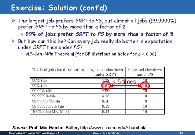
Exercise: Solution (cont’d) Ø The largest job prefers SRPT to PS, but almost all jobs (99. 9999%) prefer SRPT to PS by more than a factor of 2 v 99% of jobs prefer SRPT to PS by more than a factor of 5 Ø But how can this be? Can every job really do better in expectation under SRPT than under PS? v All-Can-Win Theorem! (for BP distribution holds for ρ < 0. 96) < 5 times Source: Prof. Mor Harchol-Balter, http: //www. cs. cmu. edu/~harchol/ Thrasyvoulos Spyropoulos / spyropou@eurecom. fr Eurecom, Sophia-Antipolis 25

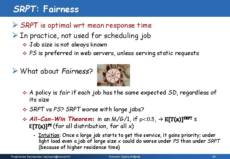
SRPT: Fairness Ø SRPT is optimal wrt mean response time Ø In practice, not used for scheduling job Job size is not always known v PS is preferred in web servers, unless serving static requests v Ø What about Fairness? v A policy is fair if each job has the same expected SD, regardless of its size v SRPT vs PS? SRPT worse with large jobs? v All-Can-Win Theorem: in an M/G/1, if ρ<0. 5, → E[T(x)]SRPT ≤ E[T(x)]PS (for all distribution, for all x) - Intuition: Once a large job starts to get the service, it gains priority; under light load even a job of large size x could do worse under PS than under SRPT (because of higher residence time) Thrasyvoulos Spyropoulos / spyropou@eurecom. fr Eurecom, Sophia-Antipolis 26

Summary on scheduling single server (M/G/1): E[T] Load r <1 Poisson arrival process Let’s order the policies based on E[T]: LOW E[T] SRPT OPT for all arrival sequences < ü Smart scheduling greatly improves mean response time (e. g. , SRPT) HIGH E[T] üLAS Variability of < PSjob size < distribution SJF < is FCFS key Requires D. F. R. (Decreasing Failure Rate) Insensitive to E[S 2] Surprisingly bad: (E[S 2] term) ~E[S 2] (shorts caught behind longs) No “Starvation!” Even the biggest jobs prefer SRPT to PS Source: Prof. Mor Harchol-Balter, http: //www. cs. cmu. edu/~harchol/ Thrasyvoulos Spyropoulos / spyropou@eurecom. fr Eurecom, Sophia-Antipolis 27

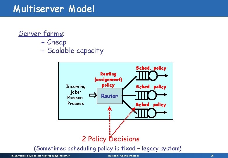
Multiserver Model Server farms: + Cheap + Scalable capacity Incoming jobs: Poisson Process Routing (assignment) policy Sched. policy Router Sched. policy 2 Policy Decisions (Sometimes scheduling policy is fixed – legacy system) Thrasyvoulos Spyropoulos / spyropou@eurecom. fr Eurecom, Sophia-Antipolis 28

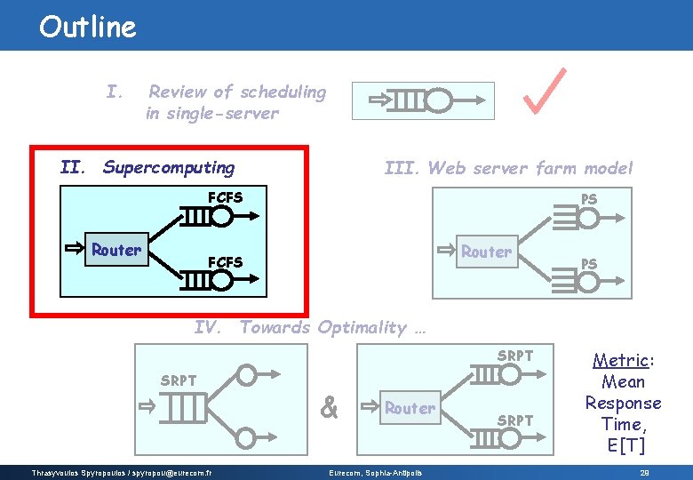
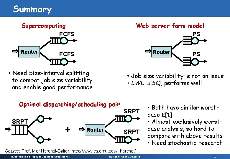
Outline I. Review of scheduling in single-server II. Supercomputing III. Web server farm model FCFS Router PS Router FCFS PS IV. Towards Optimality … SRPT Thrasyvoulos Spyropoulos / spyropou@eurecom. fr & Router Eurecom, Sophia-Antipolis SRPT Metric: Mean Response Time, E[T] 29

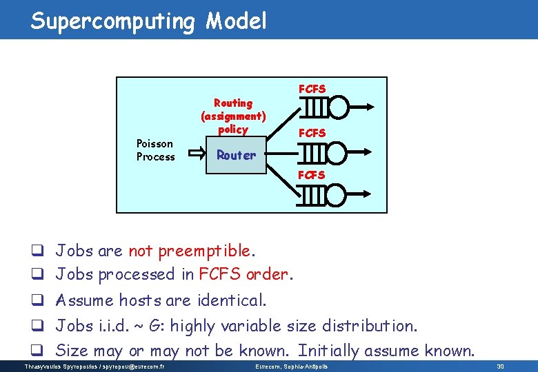
Supercomputing Model Poisson Process Routing (assignment) policy FCFS Router FCFS q Jobs are not preemptible. q Jobs processed in FCFS order. q Assume hosts are identical. q Jobs i. i. d. ~ G: highly variable size distribution. q Size may or may not be known. Initially assume known. Thrasyvoulos Spyropoulos / spyropou@eurecom. fr Eurecom, Sophia-Antipolis 30

Q: Compare Routing Policies for E[T]? Supercomputing FCFS 1. Round-Robin 2. Join-Shortest-Queue Go to host w/ fewest # jobs. Poisson Process Routing policy FCFS Router FCFS 3. Least-Work-Left Go to host with least total work. q Jobs i. i. d. ~ G: highly variable 5. Central-Queue-Shortest-Job (M/G/k/SJF) Host grabs shortest job when free. 6. Size-Interval Splitting Jobs are split up by size among hosts. Thrasyvoulos Spyropoulos / spyropou@eurecom. fr Eurecom, Sophia-Antipolis 31

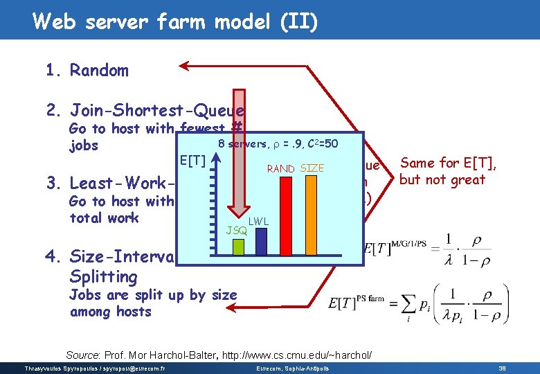
Supercomputing model (II) High E[T] 1. Round-Robin Jobs assigned to hosts (servers) in a cyclical fashion 2. Join-Shortest-Queue Go to host with fewest # jobs 3. Least-Work-Left (equalize the total work) Go to host with least total work (sum of sizes of jobs there) 4. Central-Queue-Shortest-Job (M/G/k/SJF) Host grabs shortest job when free 5. Size-Interval Splitting Low E[T] Jobs are split up by size among hosts. Each host is assigned to a size interval (e. g. , Short/Medium jobs go to the first host, Long jobs go to the second host) Thrasyvoulos Spyropoulos / spyropou@eurecom. fr Eurecom, Sophia-Antipolis Hp: Job size is known! 32

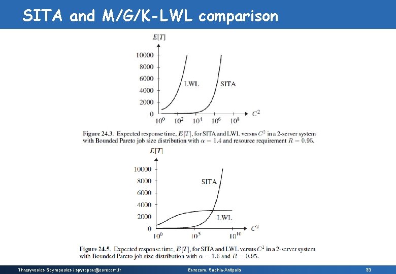
SITA and M/G/K-LWL comparison Thrasyvoulos Spyropoulos / spyropou@eurecom. fr Eurecom, Sophia-Antipolis 33

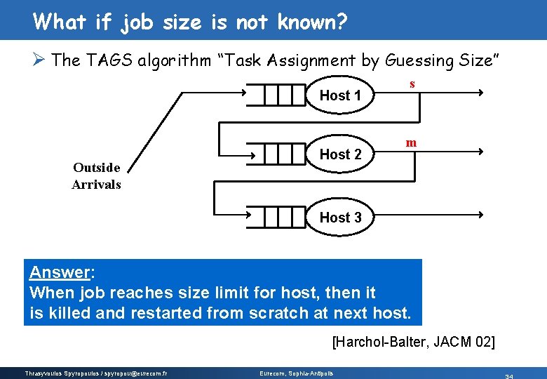
What if job size is not known? Ø The TAGS algorithm “Task Assignment by Guessing Size” Host 1 Outside Arrivals Host 2 s m Host 3 Answer: When job reaches size limit for host, then it is killed and restarted from scratch at next host. [Harchol-Balter, JACM 02] Thrasyvoulos Spyropoulos / spyropou@eurecom. fr Eurecom, Sophia-Antipolis

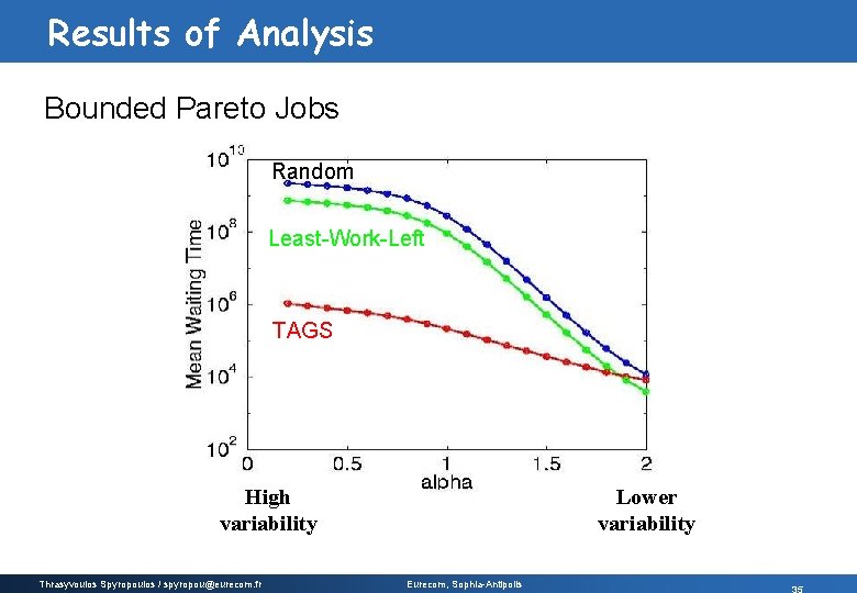
Results of Analysis Bounded Pareto Jobs Random Least-Work-Left TAGS High variability Thrasyvoulos Spyropoulos / spyropou@eurecom. fr Lower variability Eurecom, Sophia-Antipolis

Supercomputing model (III) Ø Summary v. This model is stuck with FCFS at servers. It is important to find a routing/dispatching policy that helps smalls not be stuck behind bigs → Size-Interval Splitting v By isolating small jobs, can achieve effects of smart single-server policies v Greedy routing policies (JSQ, LWL) are poor (don’t provide isolation for smalls, not good under high variability workloads) v Don’t need to know size (TAGS = Task Assignment by Guessing Size) Thrasyvoulos Spyropoulos / spyropou@eurecom. fr Eurecom, Sophia-Antipolis 36

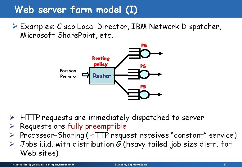
Web server farm model (I) Ø Examples: Cisco Local Director, IBM Network Dispatcher, Microsoft Share. Point, etc. PS Poisson Process Routing policy PS Router PS Ø Ø HTTP requests are immediately dispatched to server Requests are fully preemptible Processor-Sharing (HTTP request receives “constant” service) Jobs i. i. d. with distribution G (heavy tailed job size distr. for Web sites) Thrasyvoulos Spyropoulos / spyropou@eurecom. fr Eurecom, Sophia-Antipolis 37

Web server farm model (II) 1. Random 2. Join-Shortest-Queue 3. Go to host with fewest # 8 servers, r =. 9, C 2=50 jobs E[T] Shortest-Queue SIZE RAND is better (high Least-Work-Left variance distr. ) Go to host with least total work LWL Same for E[T], but not great JSQ 4. Size-Interval Splitting Jobs are split up by size among hosts Source: Prof. Mor Harchol-Balter, http: //www. cs. cmu. edu/~harchol/ Thrasyvoulos Spyropoulos / spyropou@eurecom. fr Eurecom, Sophia-Antipolis 38

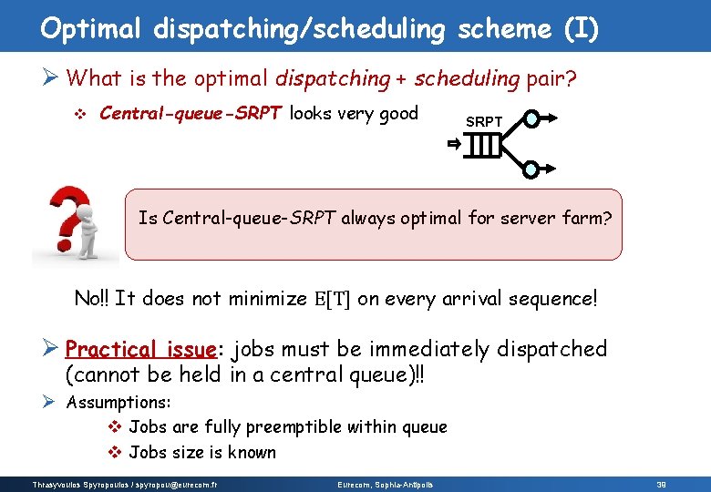
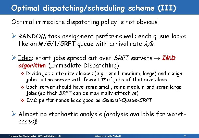
Optimal dispatching/scheduling scheme (I) Ø What is the optimal dispatching + scheduling pair? v Central-queue-SRPT looks very good SRPT Is Central-queue-SRPT always optimal for server farm? No!! It does not minimize E[T] on every arrival sequence! Ø Practical issue: jobs must be immediately dispatched (cannot be held in a central queue)!! Ø Assumptions: v Jobs are fully preemptible within queue v Jobs size is known Thrasyvoulos Spyropoulos / spyropou@eurecom. fr Eurecom, Sophia-Antipolis 39

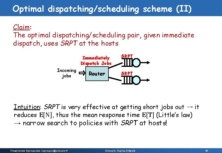
Optimal dispatching/scheduling scheme (II) Claim: The optimal dispatching/scheduling pair, given immediate dispatch, uses SRPT at the hosts Incoming jobs Immediately Dispatch Jobs SRPT Router SRPT Intuition: SRPT is very effective at getting short jobs out → it reduces E[N], thus the mean response time E[T] (Little’s law) → narrow search to policies with SRPT at hosts! Thrasyvoulos Spyropoulos / spyropou@eurecom. fr Eurecom, Sophia-Antipolis 40

Optimal dispatching/scheduling scheme (III) Optimal immediate dispatching policy is not obvious! Ø RANDOM task assignment performs well: each queue looks like an M/G/1/SRPT queue with arrival rate λ/k Ø Idea: short jobs spread out over SRPT servers → IMD algorithm (Immediate Dispatching) Divide jobs into size classes (e. g. , small, medium, large) and assign jobs to the server with fewest # of jobs of that size class v Each server should have some small, some medium and some large jobs (so that SRPT can be maximally effective) v IMD performance is as good as Central-Queue-SRPT v Ø Almost no stochastic analysis (analysis available for worstcases)! Thrasyvoulos Spyropoulos / spyropou@eurecom. fr Eurecom, Sophia-Antipolis 41

Summary Supercomputing FCFS Router Web server farm model PS Router FCFS • Need Size-interval splitting to combat job size variability and enable good performance • Job size variability is not an issue • LWL, JSQ, performs well Optimal dispatching/scheduling pair SRPT + Router PS SRPT • Both have similar worstcase E[T] • Almost exclusively worstcase analysis, so hard to compare with above results • Need stochastic research Source: Prof. Mor Harchol-Balter, http: //www. cs. cmu. edu/~harchol/ Thrasyvoulos Spyropoulos / spyropou@eurecom. fr Eurecom, Sophia-Antipolis 42

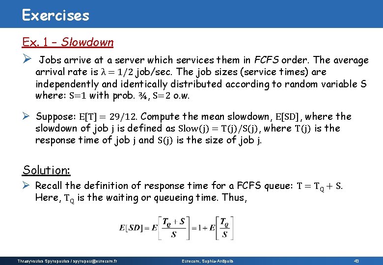
Exercises Ex. 1 – Slowdown Ø Jobs arrive at a server which services them in FCFS order. The average arrival rate is λ = 1/2 job/sec. The job sizes (service times) are independently and identically distributed according to random variable S where: S=1 with prob. ¾, S=2 o. w. Ø Suppose: E[T] = 29/12. Compute the mean slowdown, E[SD], where the slowdown of job j is defined as Slow(j) = T(j)/S(j), where T(j) is the response time of job j and S(j) is the size of job j. Solution: Ø Recall the definition of response time for a FCFS queue: T = TQ + S. Here, TQ is the waiting or queueing time. Thus, Thrasyvoulos Spyropoulos / spyropou@eurecom. fr Eurecom, Sophia-Antipolis 43

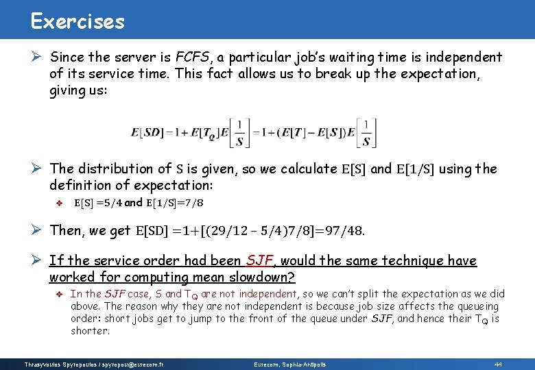
Exercises Ø Since the server is FCFS, a particular job’s waiting time is independent of its service time. This fact allows us to break up the expectation, giving us: Ø The distribution of S is given, so we calculate E[S] and E[1/S] using the definition of expectation: v E[S] =5/4 and E[1/S]=7/8 Ø Then, we get E[SD] =1+[(29/12 – 5/4)7/8]=97/48. Ø If the service order had been SJF, would the same technique have worked for computing mean slowdown? v In the SJF case, S and TQ are not independent, so we can’t split the expectation as we did above. The reason why they are not independent is because job size affects the queueing order: short jobs get to jump to the front of the queue under SJF, and hence their TQ is shorter. Thrasyvoulos Spyropoulos / spyropou@eurecom. fr Eurecom, Sophia-Antipolis 44

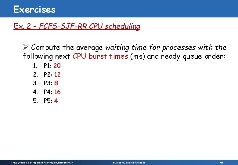
Exercises Ex. 2 – FCFS-SJF-RR CPU scheduling Ø Compute the average waiting time for processes with the following next CPU burst times (ms) and ready queue order: 1. 2. 3. 4. 5. P 1: 20 P 2: 12 P 3: 8 P 4: 16 P 5: 4 Thrasyvoulos Spyropoulos / spyropou@eurecom. fr Eurecom, Sophia-Antipolis 45

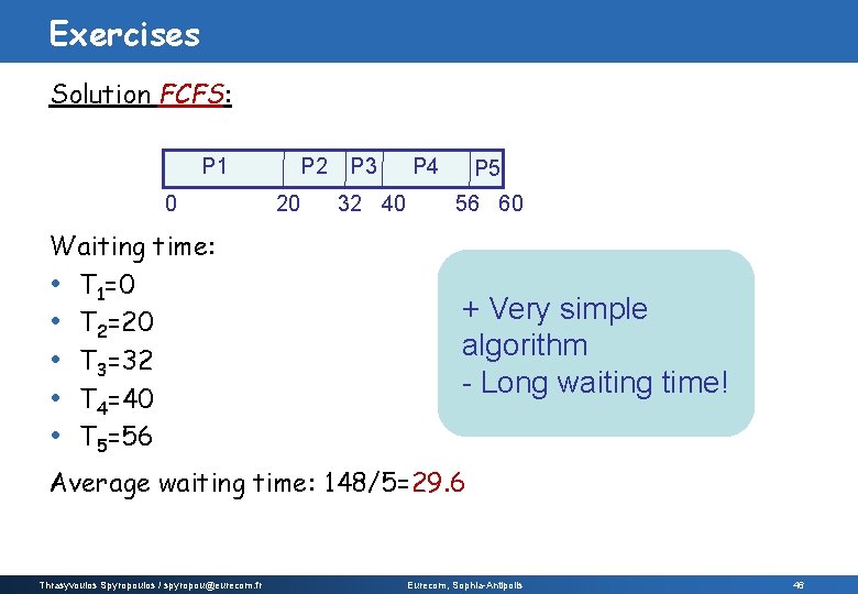
Exercises Solution FCFS: P 1 0 Waiting time: • T 1=0 • T 2=20 • T 3=32 • T 4=40 • T 5=56 P 2 20 P 3 32 40 P 4 P 5 56 60 + Very simple algorithm - Long waiting time! Average waiting time: 148/5=29. 6 Thrasyvoulos Spyropoulos / spyropou@eurecom. fr Eurecom, Sophia-Antipolis 46

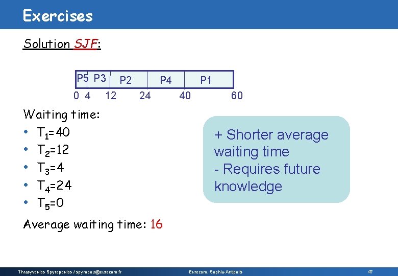
Exercises Solution SJF: P 5 P 3 0 4 P 2 12 P 4 24 Waiting time: • T 1=40 • T 2=12 • T 3=4 • T 4=24 • T 5=0 P 1 40 60 + Shorter average waiting time - Requires future knowledge Average waiting time: 16 Thrasyvoulos Spyropoulos / spyropou@eurecom. fr Eurecom, Sophia-Antipolis 47

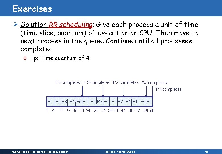
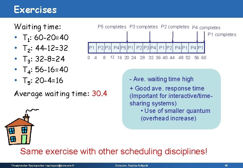
Exercises Ø Solution RR scheduling: Give each process a unit of time (time slice, quantum) of execution on CPU. Then move to next process in the queue. Continue until all processes completed. v Hp: Time quantum of 4. P 5 completes P 3 completes P 2 completes P 4 completes P 1 P 2 P 3 P 4 P 5 P 1 P 2 P 3 P 4 P 1 P 2 P 4 P 1 0 4 8 12 16 20 24 Thrasyvoulos Spyropoulos / spyropou@eurecom. fr 28 32 36 40 44 48 52 56 60 Eurecom, Sophia-Antipolis 48

Exercises Waiting time: • T 1: 60 -20=40 • T 2: 44 -12=32 • T 3: 32 -8=24 • T 4: 56 -16=40 • T 5: 20 -4=16 P 5 completes P 3 completes P 2 completes P 4 completes P 1 P 2 P 3 P 4 P 5 P 1 P 2 P 3 P 4 P 1 P 2 P 4 P 1 0 4 8 Average waiting time: 30. 4 12 16 20 24 28 32 36 40 44 48 52 56 60 - Ave. waiting time high + Good ave. response time (Important for interactive/timesharing systems) • Use of smaller quantum (overhead increase) Same exercise with other scheduling disciplines! Thrasyvoulos Spyropoulos / spyropou@eurecom. fr Eurecom, Sophia-Antipolis 49

Exercises Ex. 3 - LCFS Derive the mean queueing time E[TQ]LCFS. Derive this by conditioning on whether an arrival finds the system busy or idle. Solution: Ø With probability 1 − ρ, the arrival finds the system idle. In that case E[TQ] = 0. Ø With probability ρ, the arrival finds the system busy and has to wait for the whole busy period started by the job in service. Ø The job in service has remaining size Se. Thus the arrival has to wait for the expected duration of a busy period started by Se, which we denote by E[B(Se)] = E[Se]/(1−ρ). Thrasyvoulos Spyropoulos / spyropou@eurecom. fr Eurecom, Sophia-Antipolis 50

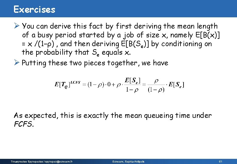
Exercises Ø You can derive this fact by first deriving the mean length of a busy period started by a job of size x, namely E[B(x)] = x /(1−ρ) , and then deriving E[B(Se)] by conditioning on the probability that Se equals x. Ø Putting these two pieces together, we have As expected, this is exactly the mean queueing time under FCFS. Thrasyvoulos Spyropoulos / spyropou@eurecom. fr Eurecom, Sophia-Antipolis 51

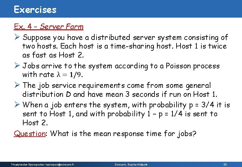
Exercises Ex. 4 – Server Farm Ø Suppose you have a distributed server system consisting of two hosts. Each host is a time-sharing host. Host 1 is twice as fast as Host 2. Ø Jobs arrive to the system according to a Poisson process with rate λ = 1/9. Ø The job service requirements come from some general distribution D and have mean 3 seconds if run on Host 1. Ø When a job enters the system, with probability p = 3/4 it is sent to Host 1, and with probability 1 − p = 1/4 is sent to Host 2. Question: What is the mean response time for jobs? Thrasyvoulos Spyropoulos / spyropou@eurecom. fr Eurecom, Sophia-Antipolis 52

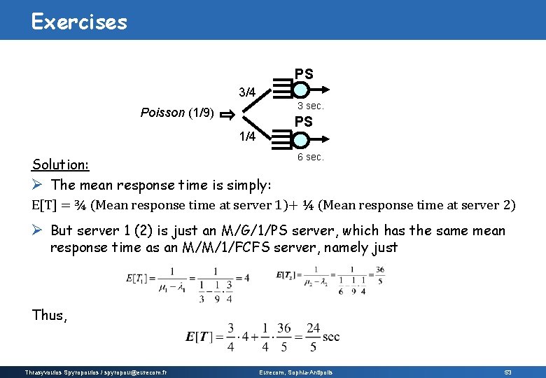
Exercises PS 3/4 3 sec. Poisson (1/9) 1/4 PS 6 sec. Solution: Ø The mean response time is simply: E[T] = ¾ (Mean response time at server 1)+ ¼ (Mean response time at server 2) Ø But server 1 (2) is just an M/G/1/PS server, which has the same mean response time as an M/M/1/FCFS server, namely just Thus, Thrasyvoulos Spyropoulos / spyropou@eurecom. fr Eurecom, Sophia-Antipolis 53

54

55

56