Lecture 4 Chapter 4 Linear Models for Correlated

Lecture 4 (Chapter 4)

Linear Models for Correlated Data We aim to develop a general linear model framework for longitudinal data, in which the inference we make about the parameters of interest recognize the likely correlation structure of the data. There are two ways of achieving this: 1. To build explicit parametric models of the covariance structure 2. To use methods of inference which are robust to misspecification of the covariance structure

General Linear Models for Correlated Data: Examples • Uniform Correlation Model – One-sample repeated measures ANOVA • Growth Model • Exponential Correlation Model • Autoregressive Model of Order 1

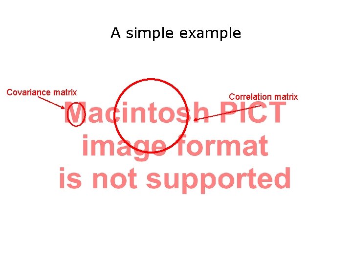
A simple example Covariance matrix Correlation matrix

Notation: Balanced Data

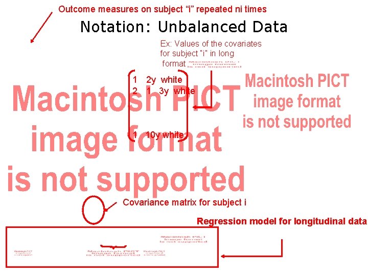
Outcome measures on subject “i” repeated ni times Notation: Unbalanced Data Ex: Values of the covariates for subject “i” in long format 1 2 y white 2 1 3 y white 1 10 y white Covariance matrix for subject i Regression model for longitudinal data

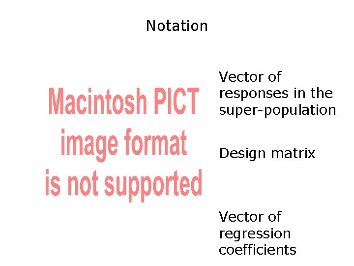
Notation Vector of responses in the super-population Design matrix Vector of regression coefficients

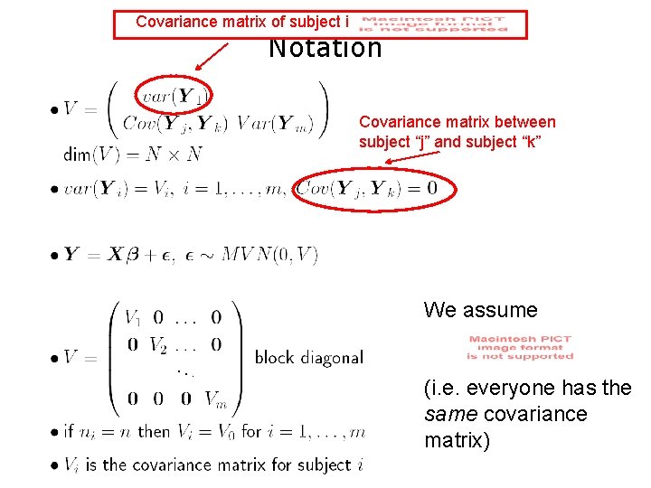
Covariance matrix of subject i Notation Covariance matrix between subject “j” and subject “k” We assume (i. e. everyone has the same covariance matrix)

Covariates may be:

Covariates may be… (cont’d)

General Linear Model with Correlated Errors Balanced Data Nx 1 (Nxp)x(px 1)(Nx. N)

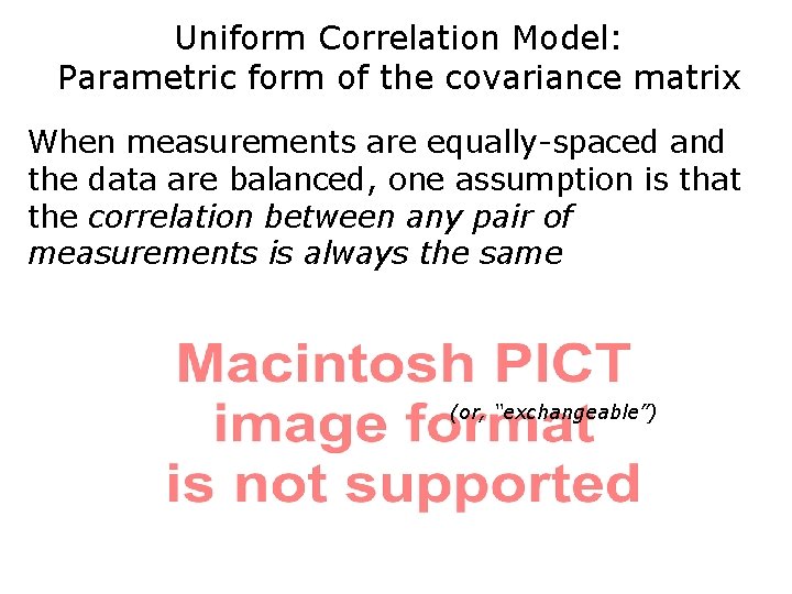
Uniform Correlation Model: Parametric form of the covariance matrix When measurements are equally-spaced and the data are balanced, one assumption is that the correlation between any pair of measurements is always the same (or, “exchangeable”)

Example: Weight of Pigs

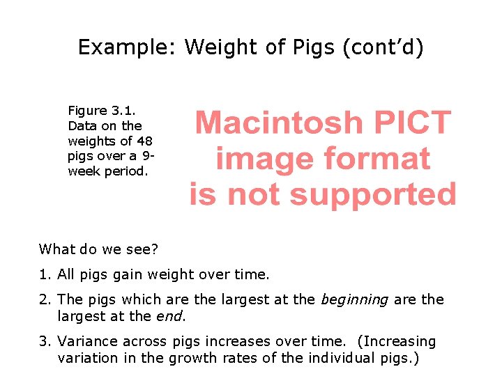
Example: Weight of Pigs (cont’d) Figure 3. 1. Data on the weights of 48 pigs over a 9 week period. What do we see? 1. All pigs gain weight over time. 2. The pigs which are the largest at the beginning are the largest at the end. 3. Variance across pigs increases over time. (Increasing variation in the growth rates of the individual pigs. )

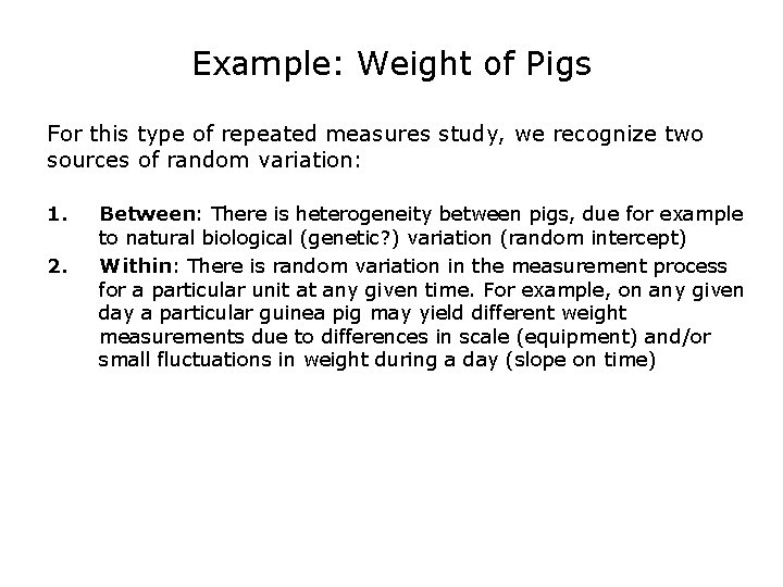
Example: Weight of Pigs For this type of repeated measures study, we recognize two sources of random variation: 1. 2. Between: There is heterogeneity between pigs, due for example to natural biological (genetic? ) variation (random intercept) Within: There is random variation in the measurement process for a particular unit at any given time. For example, on any given day a particular guinea pig may yield different weight measurements due to differences in scale (equipment) and/or small fluctuations in weight during a day (slope on time)

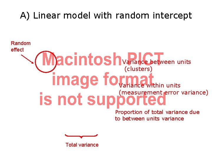
A) Linear model with random intercept Random effect Variance between units (clusters) Variance within units (measurement error variance) Proportion of total variance due to between units variance Total variance

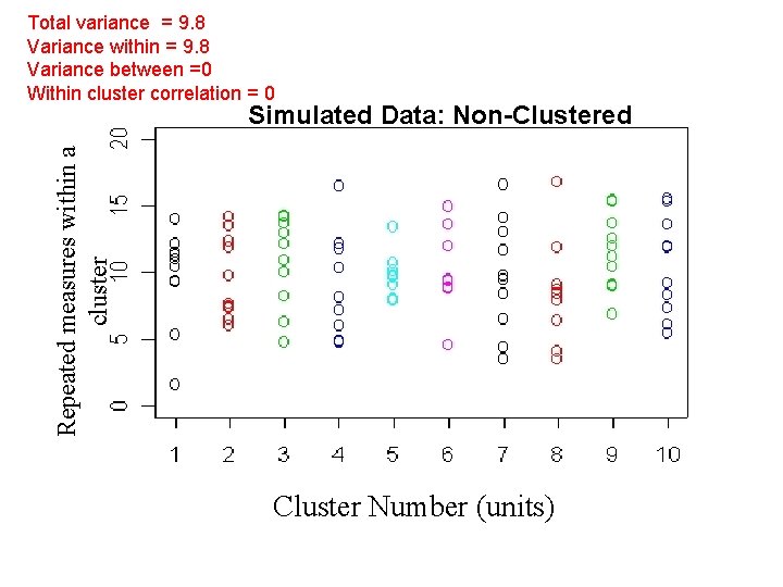
Total variance = 9. 8 Variance within = 9. 8 Variance between =0 Within cluster correlation = 0 Repeated measures within a cluster Simulated Data: Non-Clustered Cluster Number (units)

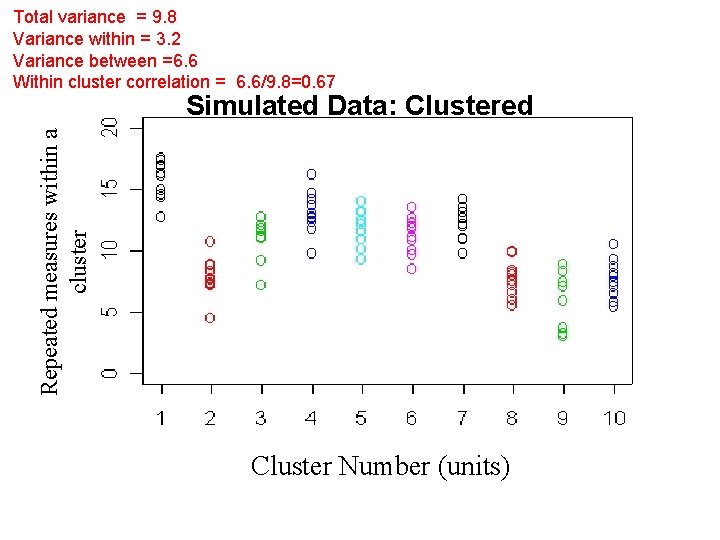
Total variance = 9. 8 Variance within = 3. 2 Variance between =6. 6 Within cluster correlation = 6. 6/9. 8=0. 67 Repeated measures within a cluster Simulated Data: Clustered Cluster Number (units)

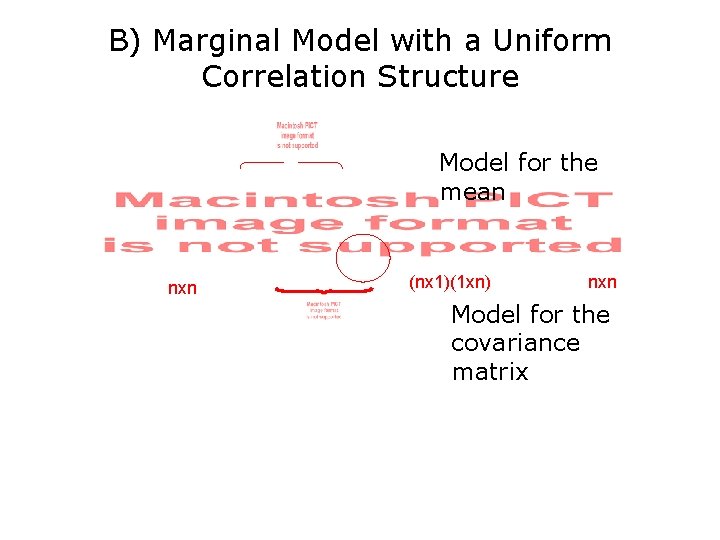
B) Marginal Model with a Uniform Correlation Structure Model for the mean nxn (nx 1)(1 xn) nxn Model for the covariance matrix

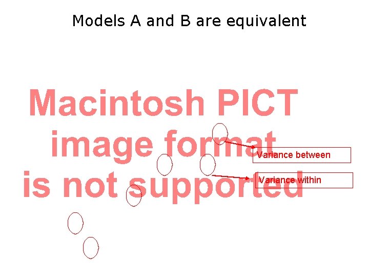
Models A and B are equivalent Variance between Variance within

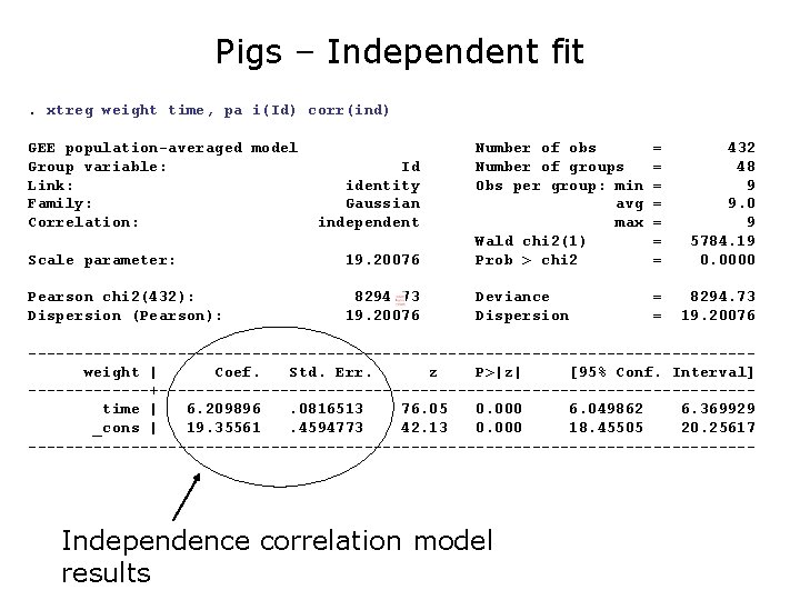
Pigs – Independent fit. xtreg weight time, pa i(Id) corr(ind) GEE population-averaged model Group variable: Link: Family: Correlation: Scale parameter: 19. 20076 Number of obs Number of groups Obs per group: min avg max Wald chi 2(1) Prob > chi 2 Pearson chi 2(432): Dispersion (Pearson): 8294. 73 19. 20076 Deviance Dispersion Id identity Gaussian independent = = = = 432 48 9 9. 0 9 5784. 19 0. 0000 = = 8294. 73 19. 20076 ---------------------------------------weight | Coef. Std. Err. z P>|z| [95% Conf. Interval] -------+--------------------------------time | 6. 209896. 0816513 76. 05 0. 000 6. 049862 6. 369929 _cons | 19. 35561. 4594773 42. 13 0. 000 18. 45505 20. 25617 --------------------------------------- Independence correlation model results

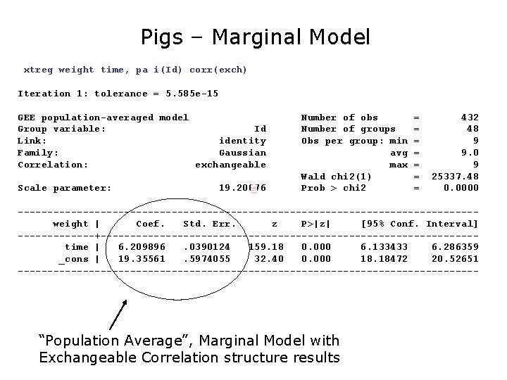
Pigs – Marginal Model xtreg weight time, pa i(Id) corr(exch) Iteration 1: tolerance = 5. 585 e-15 GEE population-averaged model Group variable: Id Link: identity Family: Gaussian Correlation: exchangeable Scale parameter: 19. 20076 Number of obs Number of groups Obs per group: min avg max Wald chi 2(1) Prob > chi 2 = = = = 432 48 9 9. 0 9 25337. 48 0. 0000 ---------------------------------------weight | Coef. Std. Err. z P>|z| [95% Conf. Interval] -------+--------------------------------time | 6. 209896. 0390124 159. 18 0. 000 6. 133433 6. 286359 _cons | 19. 35561. 5974055 32. 40 0. 000 18. 18472 20. 52651 --------------------------------------- “Population Average”, Marginal Model with Exchangeable Correlation structure results

Marginal Model E[ Yi ] = β 0+ β 1 time

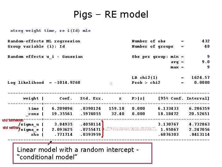
Pigs – RE model xtreg weight time, re i(Id) mle Random-effects ML regression Group variable (i): Id Number of obs Number of groups = = 432 48 Random effects u_i ~ Gaussian Obs per group: min = avg = max = 9 9. 0 9 Log likelihood = -1014. 9268 LR chi 2(1) Prob > chi 2 = = 1624. 57 0. 0000 ---------------------------------------weight | Coef. Std. Err. z P>|z| [95% Conf. Interval] -------+--------------------------------time | 6. 209896. 0390124 159. 18 0. 000 6. 133433 6. 286359 _cons | 19. 35561. 5974055 32. 40 0. 000 18. 18472 20. 52651 std-------+--------------------------------between /sigma_u | 3. 84935. 4058114 3. 130767 4. 732863 std within/sigma_e | 2. 093625. 0755471 1. 95067 2. 247056 rho |. 771714. 0393959. 6876303. 8413114 --------------------------------------- Linear model with a random intercept “conditional model”

Random Effects Model E[ Yi | Ui] = β 0+ β 1 time + Ui E[ Yi ] = β 0+ β 1 time

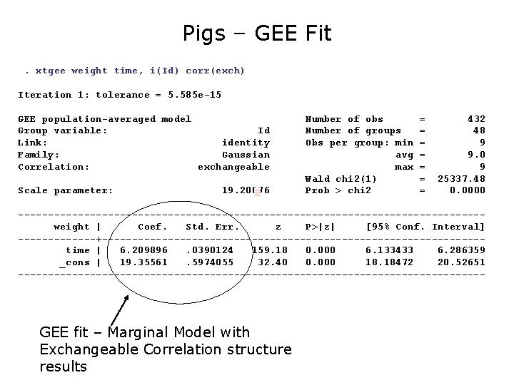
Pigs – GEE Fit. xtgee weight time, i(Id) corr(exch) Iteration 1: tolerance = 5. 585 e-15 GEE population-averaged model Group variable: Id Link: identity Family: Gaussian Correlation: exchangeable Scale parameter: 19. 20076 Number of obs Number of groups Obs per group: min avg max Wald chi 2(1) Prob > chi 2 = = = = 432 48 9 9. 0 9 25337. 48 0. 0000 ---------------------------------------weight | Coef. Std. Err. z P>|z| [95% Conf. Interval] -------+--------------------------------time | 6. 209896. 0390124 159. 18 0. 000 6. 133433 6. 286359 _cons | 19. 35561. 5974055 32. 40 0. 000 18. 18472 20. 52651 --------------------------------------- GEE fit – Marginal Model with Exchangeable Correlation structure results

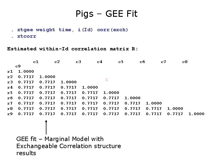
Pigs – GEE Fit. xtgee weight time, i(Id) corr(exch). xtcorr Estimated within-Id correlation matrix R: c 1 r 2 r 3 r 4 r 5 r 6 r 7 r 8 r 9 c 9 1. 0000 0. 7717 0. 7717 c 2 1. 0000 0. 7717 0. 7717 c 3 1. 0000 0. 7717 c 4 1. 0000 0. 7717 c 5 1. 0000 0. 7717 GEE fit – Marginal Model with Exchangeable Correlation structure results c 6 1. 0000 0. 7717 c 7 1. 0000 0. 7717 c 8 1. 0000 0. 7717 1. 0000

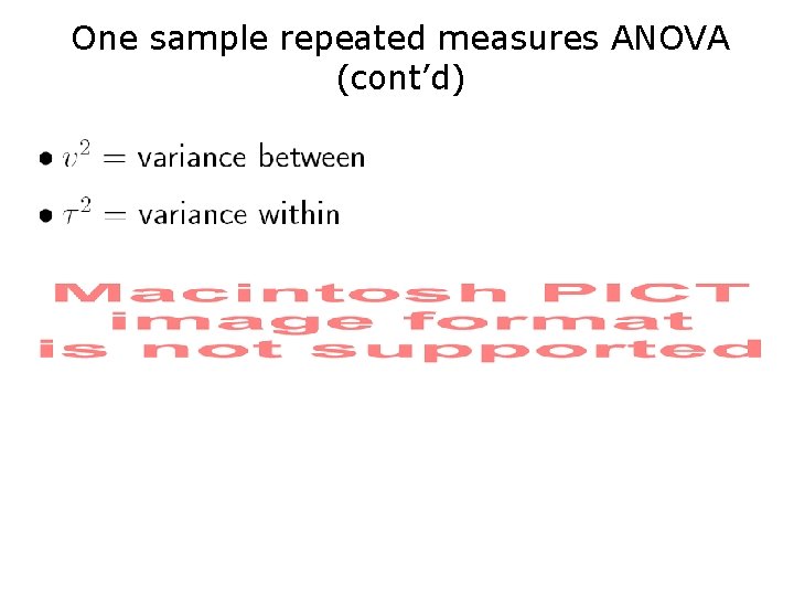
One sample repeated measures ANOVA

One sample repeated measures ANOVA (cont’d)

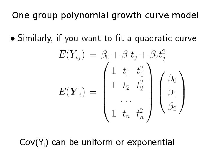
One group polynomial growth curve model

One group polynomial growth curve model Cov(Yi) can be uniform or exponential

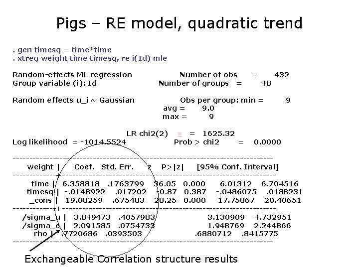
Pigs – RE model, quadratic trend. gen timesq = time*time. xtreg weight timesq, re i(Id) mle Random-effects ML regression Group variable (i): Id Random effects u_i ~ Gaussian Log likelihood = -1014. 5524 Number of obs Number of groups = = 48 432 Obs per group: min = avg = 9. 0 max = 9 LR chi 2(2) = 1625. 32 Prob > chi 2 = 9 0. 0000 ---------------------------------------weight | Coef. Std. Err. z P>|z| [95% Conf. Interval] -------+--------------------------------time | 6. 358818. 1763799 36. 05 0. 000 6. 01312 6. 704516 timesq | -. 0148922. 017202 -0. 87 0. 387 -. 0486075. 0188231 _cons | 19. 08259. 675483 28. 25 0. 000 17. 75867 20. 40651 -------+--------------------------------/sigma_u | 3. 849473. 4057983 3. 130909 4. 732951 /sigma_e | 2. 091585. 0754733 1. 948769 2. 244866 rho |. 7720686. 0393503. 6880712. 8415775 --------------------------------------- Exchangeable Correlation structure results

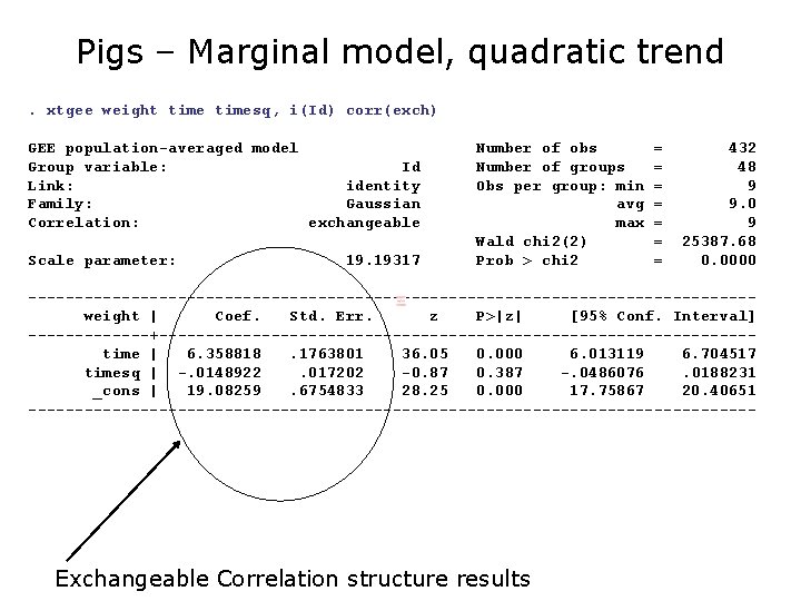
Pigs – Marginal model, quadratic trend. xtgee weight timesq, i(Id) corr(exch) GEE population-averaged model Group variable: Id Link: identity Family: Gaussian Correlation: exchangeable Scale parameter: 19. 19317 Number of obs Number of groups Obs per group: min avg max Wald chi 2(2) Prob > chi 2 = = = = 432 48 9 9. 0 9 25387. 68 0. 0000 ---------------------------------------weight | Coef. Std. Err. z P>|z| [95% Conf. Interval] -------+--------------------------------time | 6. 358818. 1763801 36. 05 0. 000 6. 013119 6. 704517 timesq | -. 0148922. 017202 -0. 87 0. 387 -. 0486076. 0188231 _cons | 19. 08259. 6754833 28. 25 0. 000 17. 75867 20. 40651 --------------------------------------- Exchangeable Correlation structure results

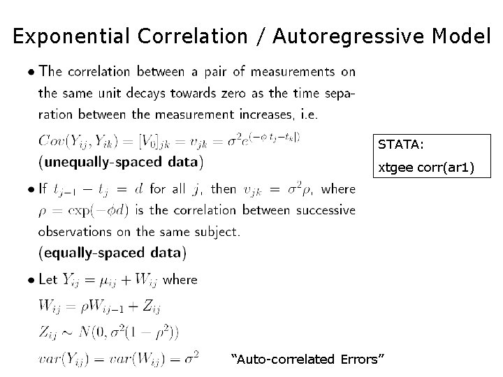
Exponential Correlation / Autoregressive Model STATA: xtgee corr(ar 1) “Auto-correlated Errors”

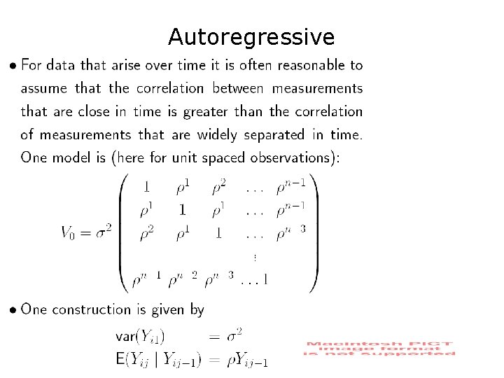
Autoregressive

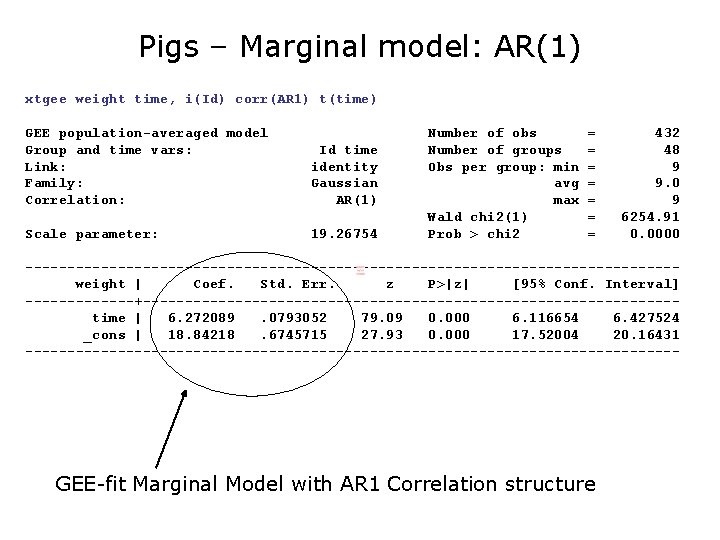
Pigs – Marginal model: AR(1) xtgee weight time, i(Id) corr(AR 1) t(time) GEE population-averaged model Group and time vars: Link: Family: Correlation: Id time identity Gaussian AR(1) Scale parameter: 19. 26754 Number of obs Number of groups Obs per group: min avg max Wald chi 2(1) Prob > chi 2 = = = = 432 48 9 9. 0 9 6254. 91 0. 0000 ---------------------------------------weight | Coef. Std. Err. z P>|z| [95% Conf. Interval] -------+--------------------------------time | 6. 272089. 0793052 79. 09 0. 000 6. 116654 6. 427524 _cons | 18. 84218. 6745715 27. 93 0. 000 17. 52004 20. 16431 --------------------------------------- GEE-fit Marginal Model with AR 1 Correlation structure

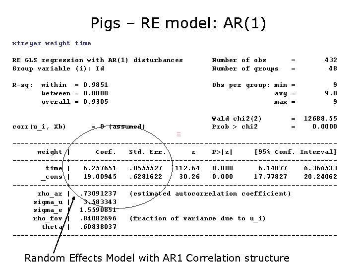
Pigs – RE model: AR(1) xtregar weight time RE GLS regression with AR(1) disturbances Group variable (i): Id Number of obs Number of groups = = 432 48 R-sq: Obs per group: min = avg = max = 9 9. 0 9 within = 0. 9851 between = 0. 0000 overall = 0. 9305 corr(u_i, Xb) = 0 (assumed) Wald chi 2(2) Prob > chi 2 = = 12688. 55 0. 0000 ---------------------------------------weight | Coef. Std. Err. z P>|z| [95% Conf. Interval] -------+--------------------------------time | 6. 257651. 0555527 112. 64 0. 000 6. 14877 6. 366533 _cons | 19. 00945. 6281622 30. 26 0. 000 17. 77827 20. 24062 -------+--------------------------------rho_ar |. 73091237 (estimated autocorrelation coefficient) sigma_u | 3. 583343 sigma_e | 1. 5590851 rho_fov |. 84082696 (fraction of variance due to u_i) theta |. 60838037 --------------------------------------- Random Effects Model with AR 1 Correlation structure

Marginal Model

Important Points • Modelling the correlation in longitudinal data is important to be able to obtain correct inferences on regression coefficients β • There are correspondences between random effect and marginal models in the linear case because the interpretation of the regression coefficients is the same as that in cross-sectional data • Correlation can be formulated in terms of subject-specific models and/or transition models • Exchangeable correlation model: subject-specific formulation • Exponential correlation model: transition model formulation

(Still More) Important Points • Three basic elements of correlation structure: • Random effects • Autocorrelation or serial dependence • Noise, measurement error • Incorporating correlation into estimation of regression models is achieved via weighted least squares

(Still More) Important Points • There are many ways of estimating correlation parameters. We will study some of these. • Correlation models can be approximate • We will call these working correlation models (“our best shot”) • Regression coefficients estimates will still be correct • We will see how to “fix up” standard errors to account for inaccuracies in correlation models