Chapter 8 Linear normal models Multiple linear regression

Chapter 8 Linear normal models

Multiple linear regression Several continuous explanatory variables, or covariates, can be measured for each observational unit. If we denote the d covariate measurements for unit i as xij, j = 1, …, d then the multiple linear regression model is defined by where the residuals are assumed to be independent and normally distributed. The regression parameters β 1, …, βd are interpreted as ordinary regression parameters: a unit change in xk corresponds to an expected change in y of βk if we assume that all other variables remain unchanged.

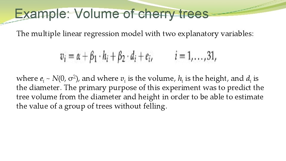
Example: Volume of cherry trees The multiple linear regression model with two explanatory variables: where ei ~ N(0, σ2), and where vi is the volume, hi is the height, and di is the diameter. The primary purpose of this experiment was to predict the tree volume from the diameter and height in order to be able to estimate the value of a group of trees without felling.

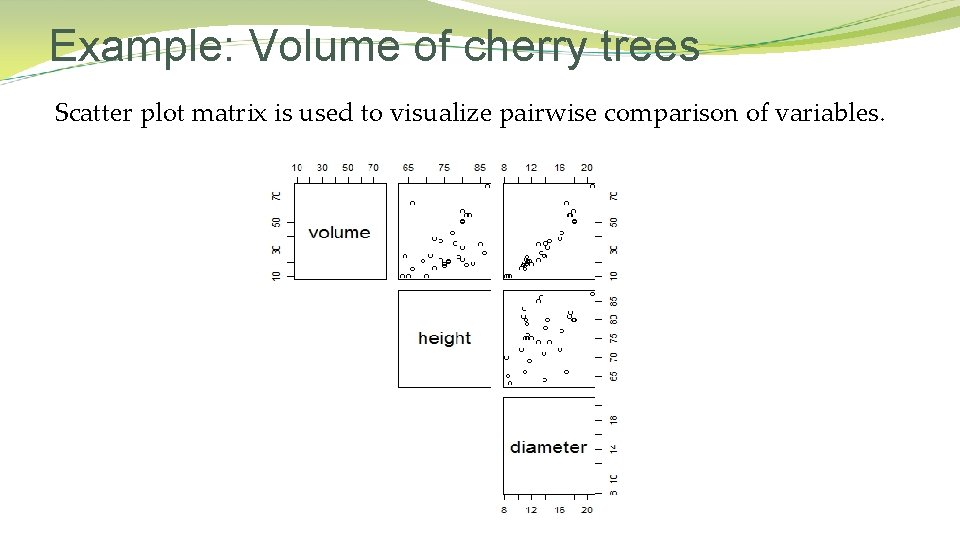
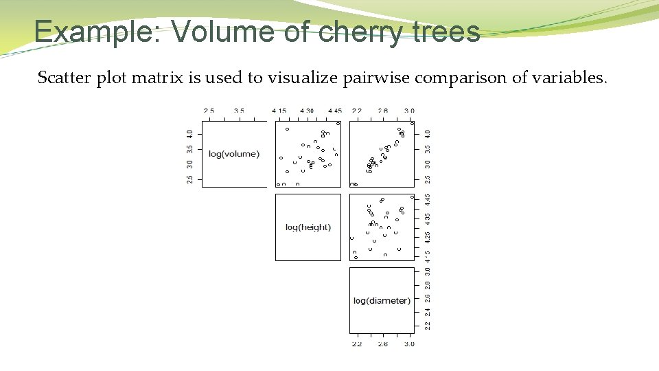
Example: Volume of cherry trees Scatter plot matrix is used to visualize pairwise comparison of variables.

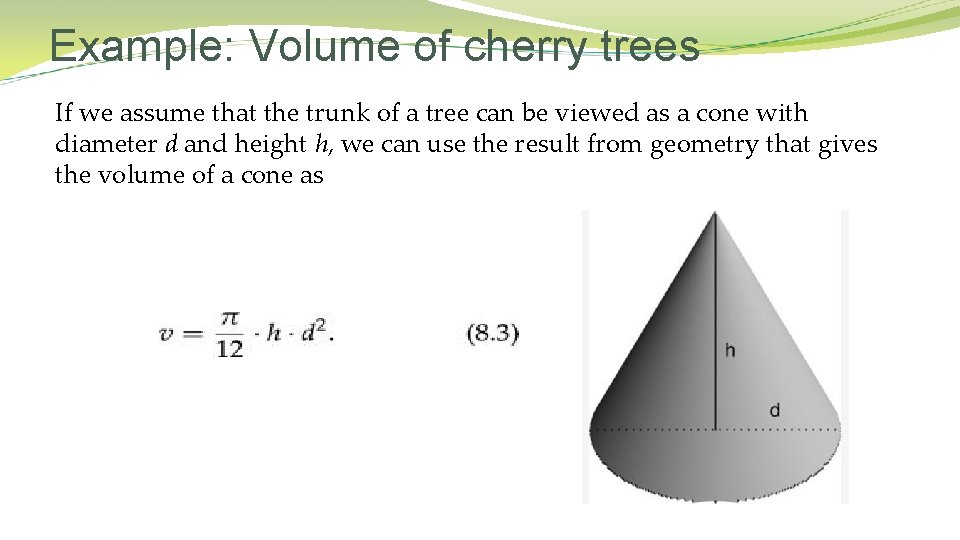
Example: Volume of cherry trees If we assume that the trunk of a tree can be viewed as a cone with diameter d and height h, we can use the result from geometry that gives the volume of a cone as

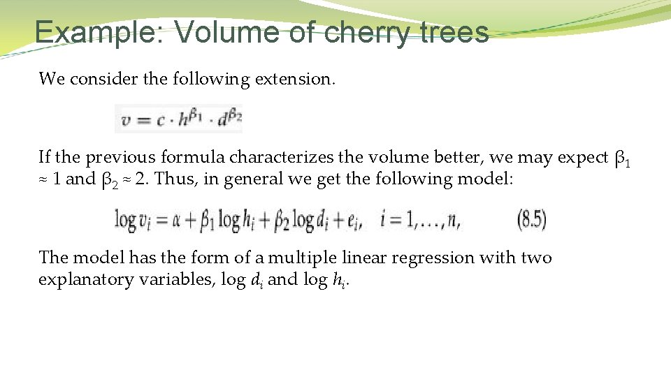
Example: Volume of cherry trees We consider the following extension. If the previous formula characterizes the volume better, we may expect β 1 ≈ 1 and β 2 ≈ 2. Thus, in general we get the following model: The model has the form of a multiple linear regression with two explanatory variables, log di and log hi.

Example: Volume of cherry trees Scatter plot matrix is used to visualize pairwise comparison of variables.

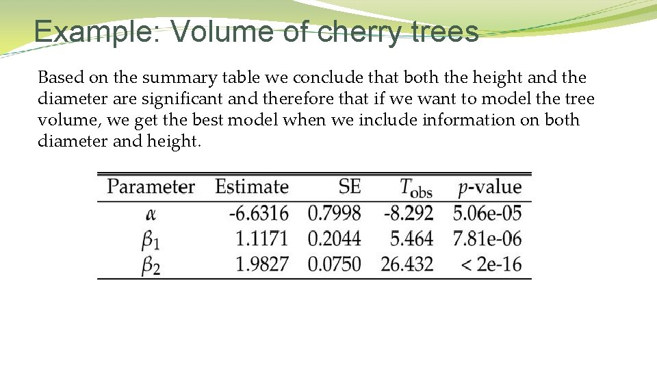
Example: Volume of cherry trees Based on the summary table we conclude that both the height and the diameter are significant and therefore that if we want to model the tree volume, we get the best model when we include information on both diameter and height.

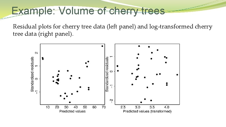
Example: Volume of cherry trees Residual plots for cherry tree data (left panel) and log-transformed cherry tree data (right panel).

Null hypotheses for coefficients The statistical model under the null hypothesis H 0: βj = 0 is a multiple linear regression model without the jth covariate, but with the other covariates remaining in the model. The test therefore examines if the jth covariate contributes to the explanation of variation in y when the association between y and other covariates has been taken into account. In the cherry tree example the hypotheses for β 1 = 0 and for β 2 = 0 have been rejected. The conclusion would be that there is association between height and volume and between diameter and volume.

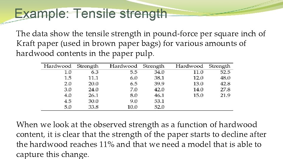
Example: Tensile strength The data show the tensile strength in pound-force per square inch of Kraft paper (used in brown paper bags) for various amounts of hardwood contents in the paper pulp. When we look at the observed strength as a function of hardwood content, it is clear that the strength of the paper starts to decline after the hardwood reaches 11% and that we need a model that is able to capture this change.

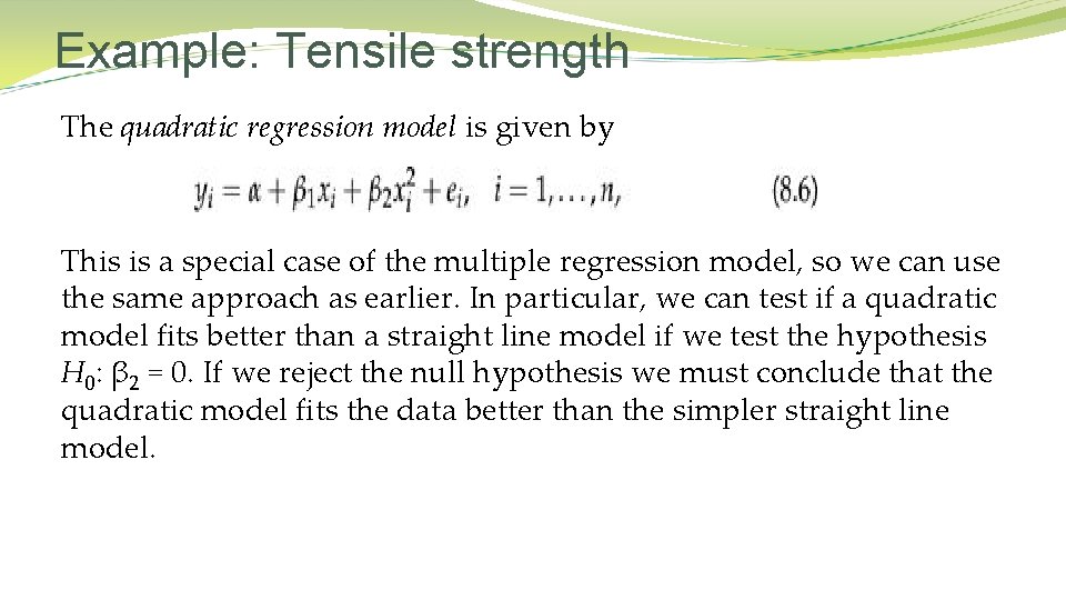
Example: Tensile strength The quadratic regression model is given by This is a special case of the multiple regression model, so we can use the same approach as earlier. In particular, we can test if a quadratic model fits better than a straight line model if we test the hypothesis H 0: β 2 = 0. If we reject the null hypothesis we must conclude that the quadratic model fits the data better than the simpler straight line model.

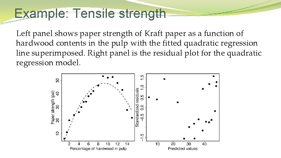
Example: Tensile strength Left panel shows paper strength of Kraft paper as a function of hardwood contents in the pulp with the fitted quadratic regression line superimposed. Right panel is the residual plot for the quadratic regression model.

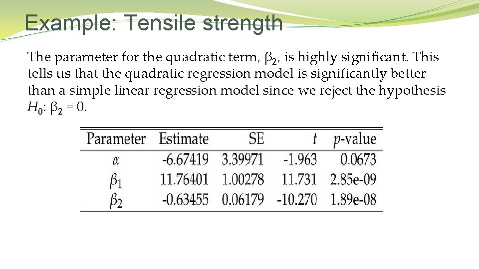
Example: Tensile strength The parameter for the quadratic term, β 2, is highly significant. This tells us that the quadratic regression model is significantly better than a simple linear regression model since we reject the hypothesis H 0: β 2 = 0.

Collinearity and multicollinearity Collinearity is a linear relationship between two explanatory variables and multicollinearity refers to the situation where two or more explanatory variables are highly correlated. For example, two covariates (e. g. , height and weight) may measure different aspects of the same thing (e. g. , size). Multicollinearity may give rise to spurious results. For example, you may find estimates with the opposite sign compared to what you would expect, unrealistically high standard errors, and insignificant effects of covariates that you would expect to be significant. The problem is that it is hard to distinguish the effect of one of the covariates from the others. The model fits more or less equally well no matter if the effect is measured through one or the other variable.

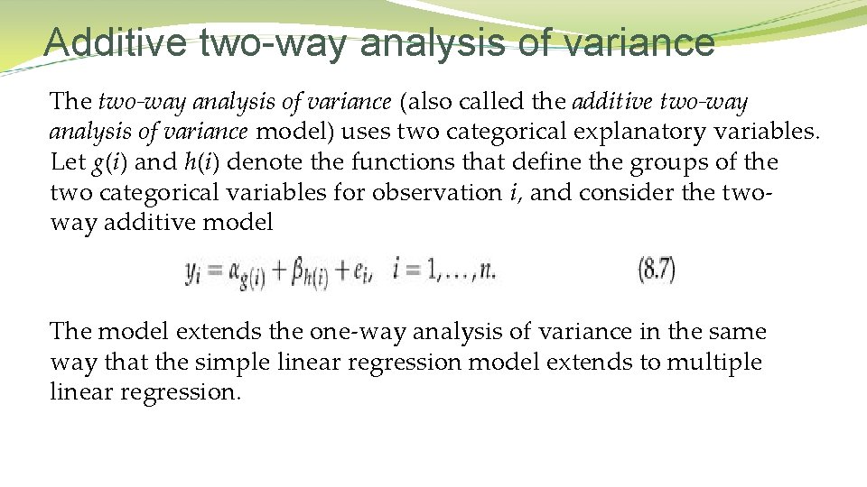
Additive two-way analysis of variance The two-way analysis of variance (also called the additive two-way analysis of variance model) uses two categorical explanatory variables. Let g(i) and h(i) denote the functions that define the groups of the two categorical variables for observation i, and consider the twoway additive model The model extends the one-way analysis of variance in the same way that the simple linear regression model extends to multiple linear regression.

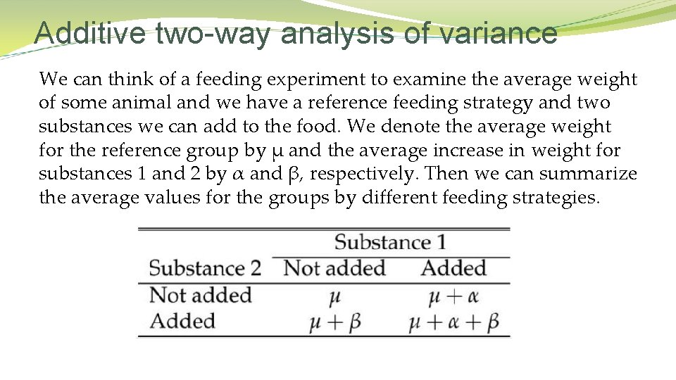
Additive two-way analysis of variance We can think of a feeding experiment to examine the average weight of some animal and we have a reference feeding strategy and two substances we can add to the food. We denote the average weight for the reference group by μ and the average increase in weight for substances 1 and 2 by α and β, respectively. Then we can summarize the average values for the groups by different feeding strategies.

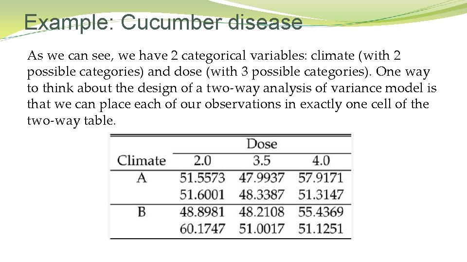
Example: Cucumber disease This study examines how the spread of a disease in cucumbers depends on climate and amount of fertilizer. Two different climates were used: (A) change to day temperature 3 hours before sunrise and (B) normal change to day temperature. Fertilizer was applied in 3 different doses: 2. 0, 3. 5, and 4. 0 units. The amount of infection on standardized plants was recorded after a number of days, and two plants were examined for each combination of climate and dose.

Example: Cucumber disease As we can see, we have 2 categorical variables: climate (with 2 possible categories) and dose (with 3 possible categories). One way to think about the design of a two-way analysis of variance model is that we can place each of our observations in exactly one cell of the two-way table.

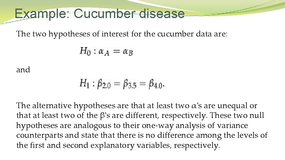
Example: Cucumber disease The two hypotheses of interest for the cucumber data are: and The alternative hypotheses are that at least two α's are unequal or that at least two of the β's are different, respectively. These two null hypotheses are analogous to their one-way analysis of variance counterparts and state that there is no difference among the levels of the first and second explanatory variables, respectively.

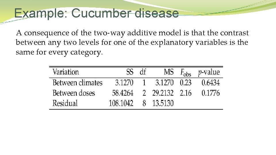
Example: Cucumber disease A consequence of the two-way additive model is that the contrast between any two levels for one of the explanatory variables is the same for every category.

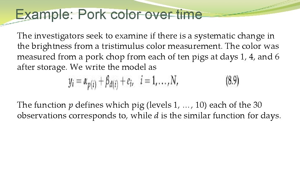
Example: Pork color over time The investigators seek to examine if there is a systematic change in the brightness from a tristimulus color measurement. The color was measured from a pork chop from each of ten pigs at days 1, 4, and 6 after storage. We write the model as The function p defines which pig (levels 1, …, 10) each of the 30 observations corresponds to, while d is the similar function for days.

Example: Pork color over time We include pig as an explanatory variable because we suspect that meat brightness might depend on which specific pig the pork was cut from. Hence, there could be an effect of “pig”, and we seek to account for that by including pig in the model even though we are not particularly interested in being able to compare any pair of pigs like, say, pig 2 and pig 7. This is called a block experiment with pigs as “blocks”. Sometimes observational units are grouped in such blocks and the observational units within a block are expected to be more similar than observations from different blocks. We expect observations taken on the same pig to be potentially more similar than observations taken on different pigs.

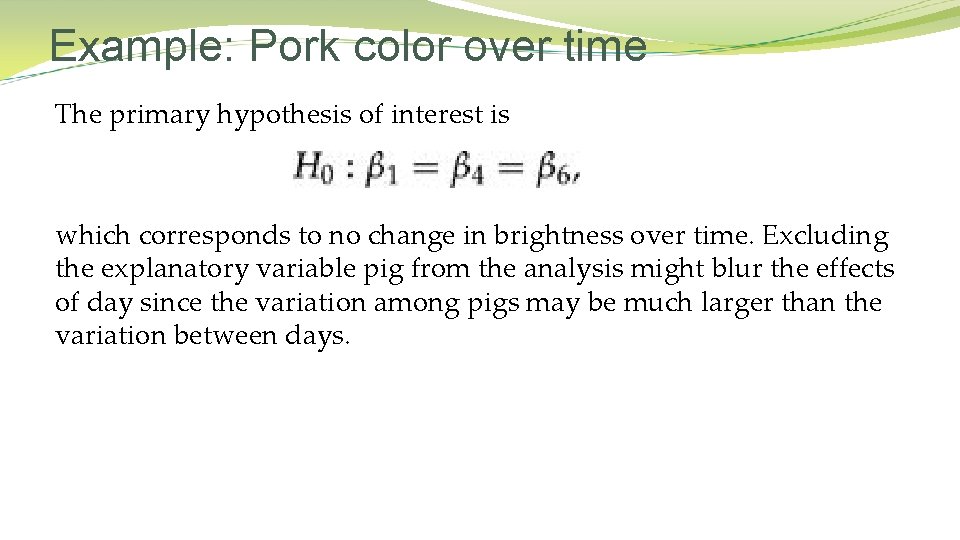
Example: Pork color over time The primary hypothesis of interest is which corresponds to no change in brightness over time. Excluding the explanatory variable pig from the analysis might blur the effects of day since the variation among pigs may be much larger than the variation between days.

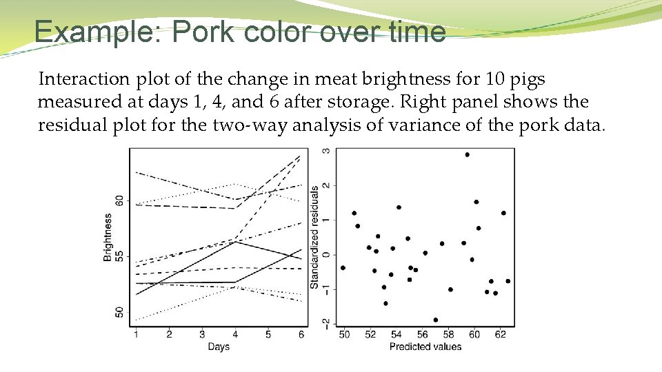
Example: Pork color over time Interaction plot of the change in meat brightness for 10 pigs measured at days 1, 4, and 6 after storage. Right panel shows the residual plot for the two-way analysis of variance of the pork data.

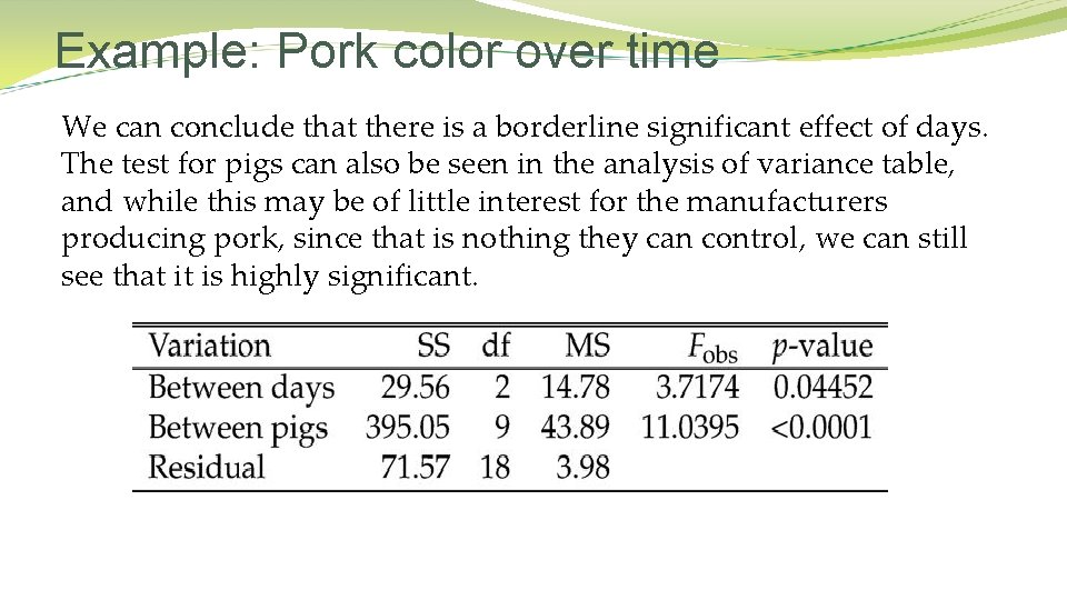
Example: Pork color over time We can conclude that there is a borderline significant effect of days. The test for pigs can also be seen in the analysis of variance table, and while this may be of little interest for the manufacturers producing pork, since that is nothing they can control, we can still see that it is highly significant.