Shengyu Zhang The Chinese University of Hong Kong

Shengyu Zhang The Chinese University of Hong Kong

Map n Intro to strategic-form games q q q n Algorithmic questions in games q q n Two forms Examples NE and CE Hardness of finding an NE and CE Congestion games Game theory applied to computer science

Part I. strategic-form games

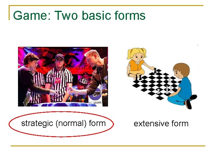
Game: Two basic forms strategic (normal) form extensive form

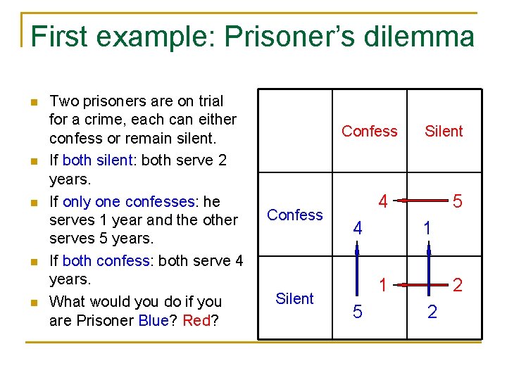
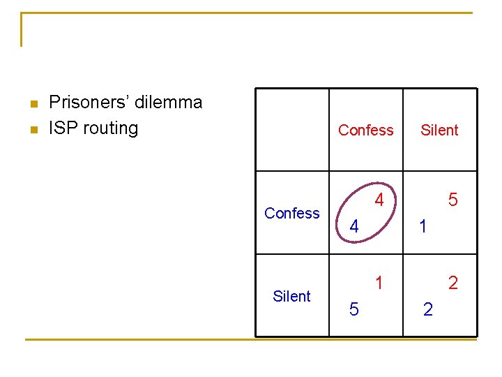
First example: Prisoner’s dilemma n n n Two prisoners are on trial for a crime, each can either confess or remain silent. If both silent: both serve 2 years. If only one confesses: he serves 1 year and the other serves 5 years. If both confess: both serve 4 years. What would you do if you are Prisoner Blue? Red? Confess Silent 4 Confess 4 5 1 5 2 2 Silent

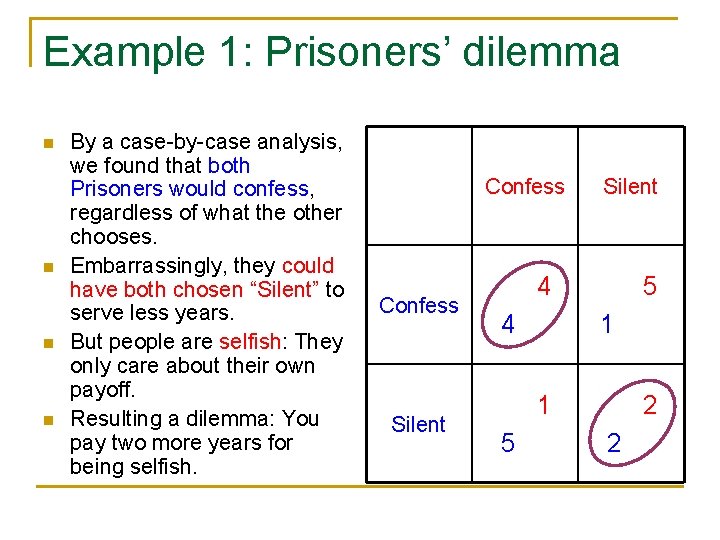
Example 1: Prisoners’ dilemma n n By a case-by-case analysis, we found that both Prisoners would confess, regardless of what the other chooses. Embarrassingly, they could have both chosen “Silent” to serve less years. But people are selfish: They only care about their own payoff. Resulting a dilemma: You pay two more years for being selfish. Confess Silent 4 Confess 4 5 1 5 2 2 Silent

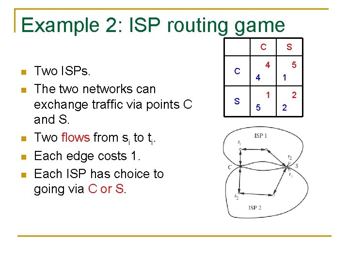
Example 2: ISP routing game n n n Two ISPs. The two networks can exchange traffic via points C and S. Two flows from si to ti. Each edge costs 1. Each ISP has choice to going via C or S. C S C 4 4 5 1 S 1 5 2 2

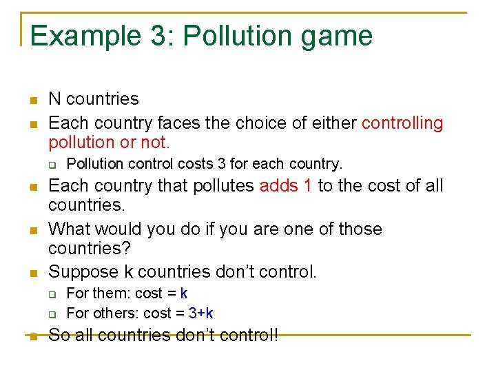
Example 3: Pollution game n n N countries Each country faces the choice of either controlling pollution or not. q n n n Each country that pollutes adds 1 to the cost of all countries. What would you do if you are one of those countries? Suppose k countries don’t control. q q n Pollution control costs 3 for each country. For them: cost = k For others: cost = 3+k So all countries don’t control!

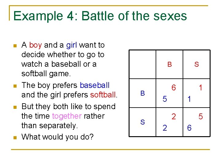
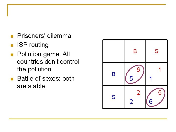
Example 4: Battle of the sexes n n A boy and a girl want to decide whether to go to watch a baseball or a softball game. The boy prefers baseball and the girl prefers softball. But they both like to spend the time together rather than separately. What would you do? B S B 6 5 1 1 S 2 2 5 6

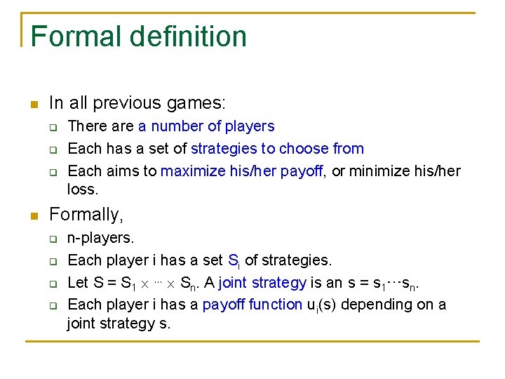
Formal definition n In all previous games: q q q n There a number of players Each has a set of strategies to choose from Each aims to maximize his/her payoff, or minimize his/her loss. Formally, q q n-players. Each player i has a set Si of strategies. Let S = S 1 ⋯ Sn. A joint strategy is an s = s 1…sn. Each player i has a payoff function ui(s) depending on a joint strategy s.

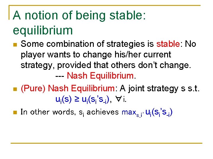
A notion of being stable: equilibrium n n n Some combination of strategies is stable: No player wants to change his/her current strategy, provided that others don’t change. --- Nash Equilibrium. (Pure) Nash Equilibrium: A joint strategy s s. t. ui(s) ≥ ui(si’s-i), ∀i. In other words, si achieves maxs_i’ui(si’s-i)

n n Prisoners’ dilemma ISP routing Confess Silent 4 Confess 4 5 1 5 2 2 Silent

n n Prisoners’ dilemma ISP routing Pollution game: All countries don’t control the pollution. Battle of sexes: both are stable. B S B 6 5 1 1 S 2 2 5 6

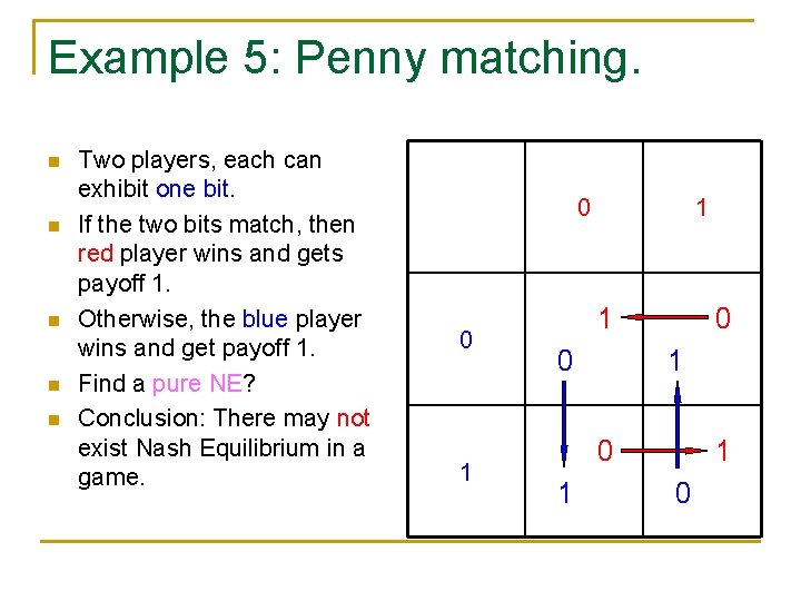
Example 5: Penny matching. n n n Two players, each can exhibit one bit. If the two bits match, then red player wins and gets payoff 1. Otherwise, the blue player wins and get payoff 1. Find a pure NE? Conclusion: There may not exist Nash Equilibrium in a game. 0 1 0 0 1 1 0

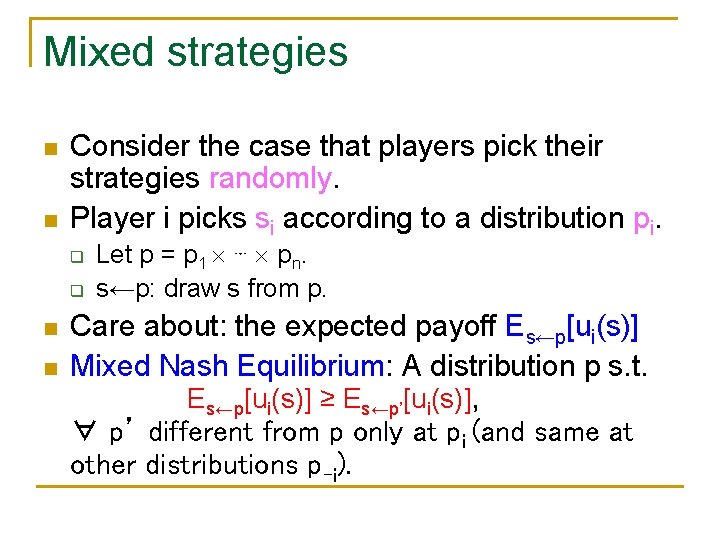
Mixed strategies n n Consider the case that players pick their strategies randomly. Player i picks si according to a distribution pi. q q n n Let p = p 1 ⋯ pn. s←p: draw s from p. Care about: the expected payoff Es←p[ui(s)] Mixed Nash Equilibrium: A distribution p s. t. Es←p[ui(s)] ≥ Es←p’[ui(s)], ∀ p’ different from p only at pi (and same at other distributions p-i).

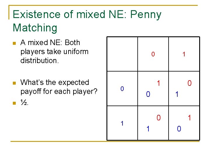
Existence of mixed NE: Penny Matching n n n A mixed NE: Both players take uniform distribution. What’s the expected payoff for each player? ½. 0 1 0 0 1 1 0

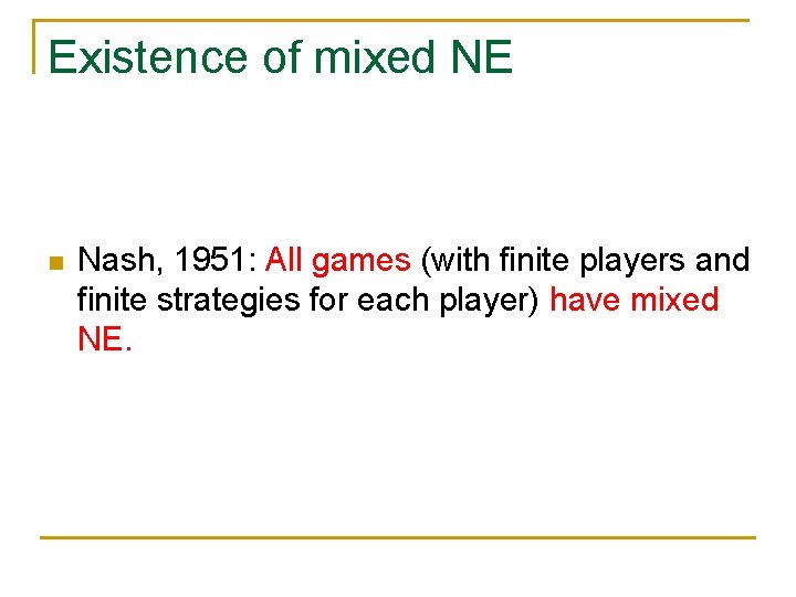
Existence of mixed NE n Nash, 1951: All games (with finite players and finite strategies for each player) have mixed NE.

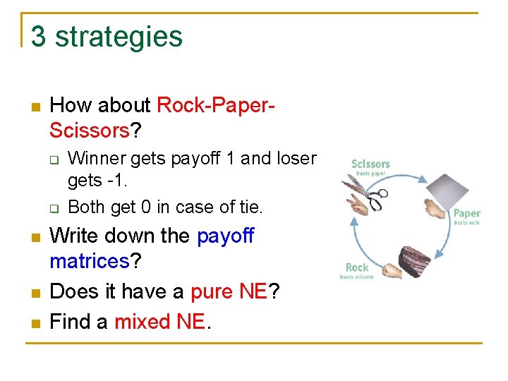
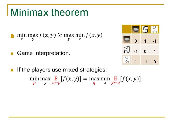
3 strategies n How about Rock-Paper. Scissors? q q n n n Winner gets payoff 1 and loser gets -1. Both get 0 in case of tie. Write down the payoff matrices? Does it have a pure NE? Find a mixed NE.

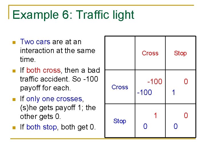
Example 6: Traffic light n n Two cars are at an interaction at the same time. If both cross, then a bad traffic accident. So -100 payoff for each. If only one crosses, (s)he gets payoff 1; the other gets 0. If both stop, both get 0. Cross Stop -100 0 Cross -100 1 Stop 1 0 0

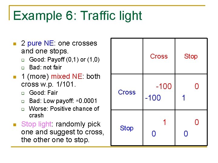
Example 6: Traffic light n 2 pure NE: one crosses and one stops. q q n 1 (more) mixed NE: both cross w. p. 1/101. q q q n Cross Good: Payoff (0, 1) or (1, 0) Bad: not fair Good: Fair Bad: Low payoff: ≃0. 0001 Worse: Positive chance of crash Stop light: randomly pick one and suggest to cross, the other one to stop. Stop -100 0 Cross -100 1 Stop 1 0 0

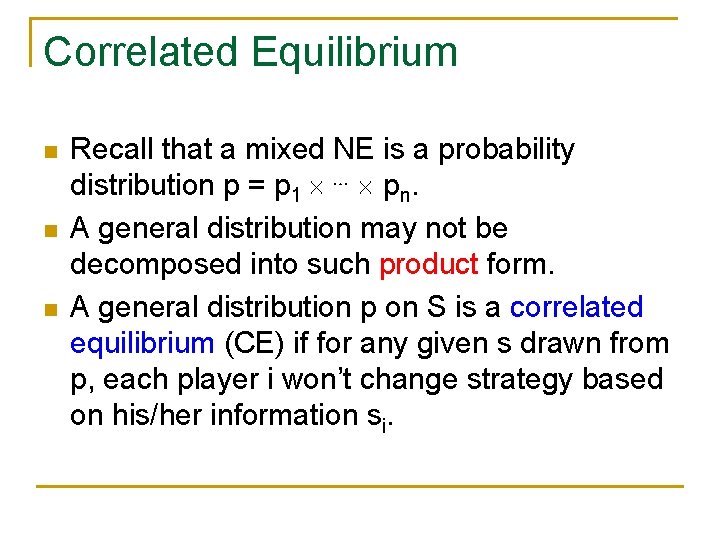
Correlated Equilibrium n n n Recall that a mixed NE is a probability distribution p = p 1 ⋯ pn. A general distribution may not be decomposed into such product form. A general distribution p on S is a correlated equilibrium (CE) if for any given s drawn from p, each player i won’t change strategy based on his/her information si.

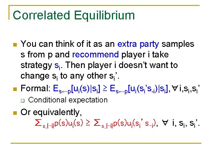
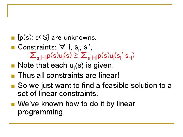
Correlated Equilibrium n n You can think of it as an extra party samples s from p and recommend player i take strategy si. Then player i doesn’t want to change si to any other si’. Formal: Es←p[ui(s)|si] ≥ Es←p[ui(si’s-i)|si], ∀i, si’ q n Conditional expectation Or equivalently, ∑s_{-i}p(s)ui(s) ≥ ∑s_{-i}p(s)ui(si’s-i), ∀ i, si’.

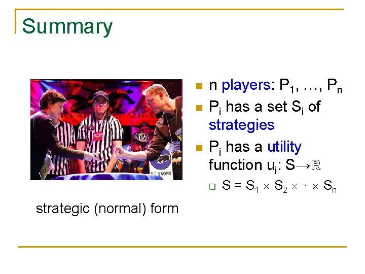
Summary n n players: P 1, …, Pn Pi has a set Si of strategies Pi has a utility function ui: S→ℝ q strategic (normal) form S = S 1 S 2 ⋯ Sn

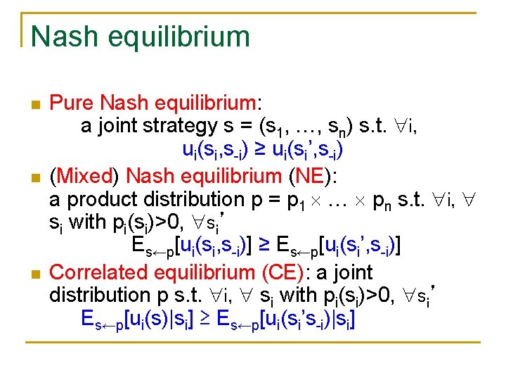
Nash equilibrium n n n Pure Nash equilibrium: a joint strategy s = (s 1, …, sn) s. t. i, ui(si, s-i) ≥ ui(si’, s-i) (Mixed) Nash equilibrium (NE): a product distribution p = p 1 … pn s. t. i, si with pi(si)>0, si’ Es←p[ui(si, s-i)] ≥ Es←p[ui(si’, s-i)] Correlated equilibrium (CE): a joint distribution p s. t. i, si with pi(si)>0, si’ Es←p[ui(s)|si] ≥ Es←p[ui(si’s-i)|si]

Part II. Algorithmic questions in games

Complexity of finding a NE and CE

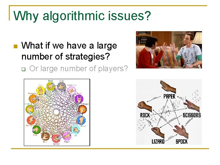
Why algorithmic issues? n What if we have a large number of strategies? q Or large number of players?

Complexity of finding a NE and CE n n n Given the utility functions, how hard is it to find one NE? No polynomial time algorithm is known to find a NE. But, there is polynomial-time algorithms for finding a correlated equilibrium.

n n n {p(s): s∊S} are unknowns. Constraints: ∀ i, si’, ∑s_{-i}p(s)ui(s) ≥ ∑s_{-i}p(s)ui(si’s-i) Note that each ui(s) is given. Thus all constraints are linear! So we just want to find a feasible solution to a set of linear constraints. We’ve known how to do it by linear programming.

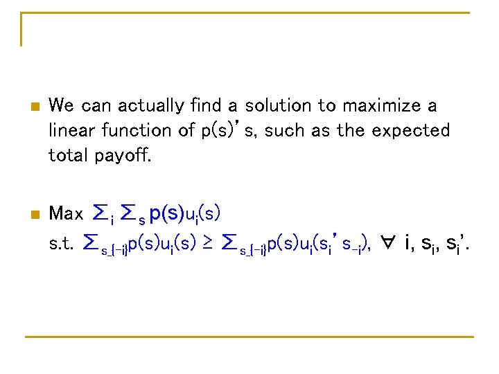
n We can actually find a solution to maximize a linear function of p(s)’s, such as the expected total payoff. n Max ∑i ∑s p(s)ui(s) s. t. ∑s_{-i}p(s)ui(s) ≥ ∑s_{-i}p(s)ui(si’s-i), ∀ i, si’.

Congestion games

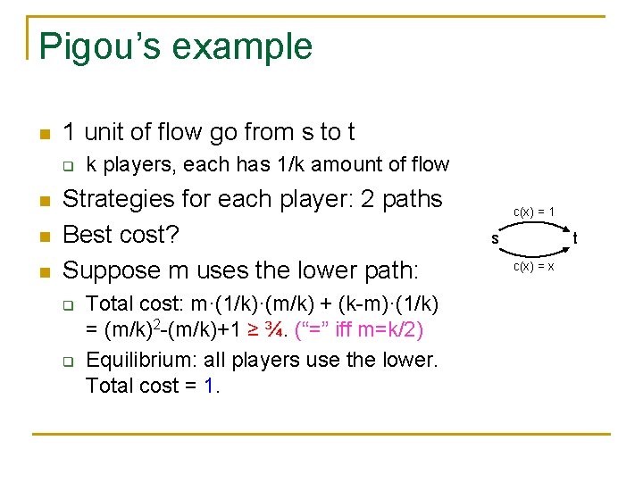
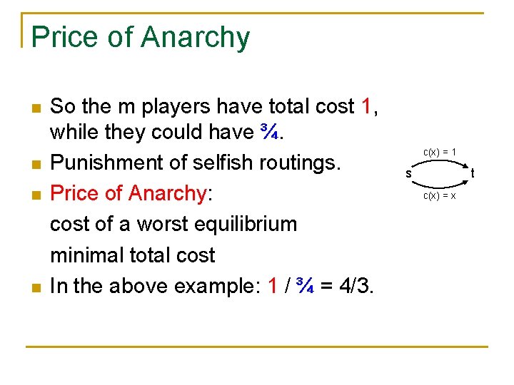
Pigou’s example n 1 unit of flow go from s to t q n n n k players, each has 1/k amount of flow Strategies for each player: 2 paths Best cost? Suppose m uses the lower path: q q Total cost: m·(1/k)·(m/k) + (k-m)·(1/k) = (m/k)2 -(m/k)+1 ≥ ¾. (“=” iff m=k/2) Equilibrium: all players use the lower. Total cost = 1. c(x) = 1 s t c(x) = x

Price of Anarchy n n So the m players have total cost 1, while they could have ¾. Punishment of selfish routings. Price of Anarchy: cost of a worst equilibrium minimal total cost In the above example: 1 / ¾ = 4/3. c(x) = 1 s t c(x) = x

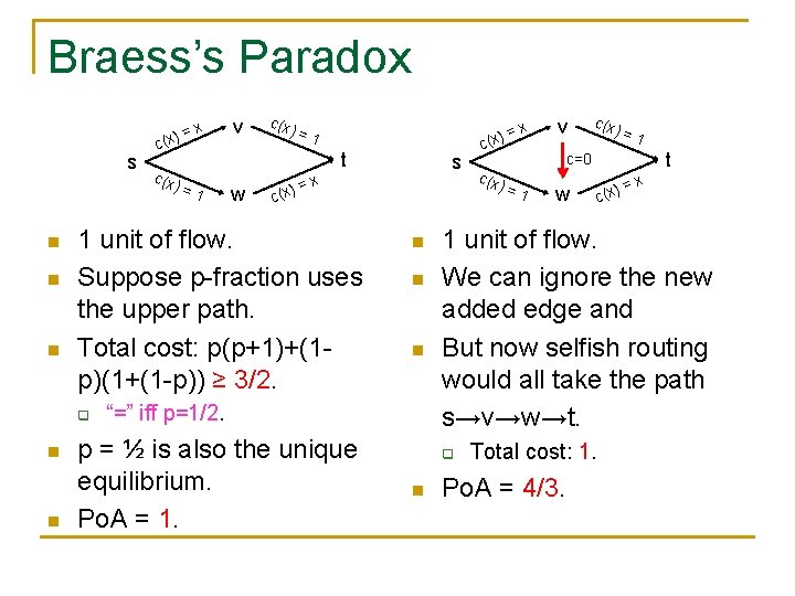
Braess’s Paradox = x (x) s c c(x) = 1 n n c(x) = x (x) = 1 t w ) = c(x s x 1 unit of flow. Suppose p-fraction uses the upper path. Total cost: p(p+1)+(1 p)(1+(1 -p)) ≥ 3/2. q n v n n n = 1 t c(x) w x ) = c(x 1 unit of flow. We can ignore the new added edge and But now selfish routing would all take the path s→v→w→t. q n c(x) c=0 = 1 “=” iff p=1/2. p = ½ is also the unique equilibrium. Po. A = 1. c v Total cost: 1. Po. A = 4/3.

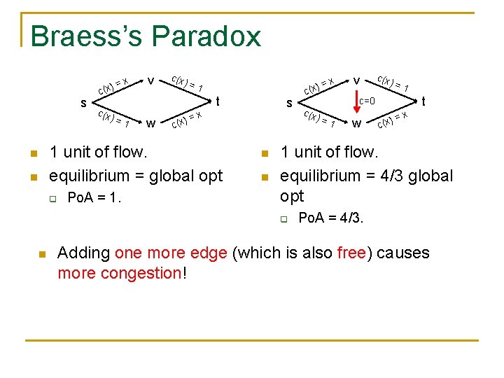
Braess’s Paradox = x (x) s c c(x) = 1 n n v c(x) t w ) = c(x Po. A = 1. s x 1 unit of flow. equilibrium = global opt q = x (x) = 1 n n c(x) = 1 t c(x) c=0 = 1 w x ) = c(x 1 unit of flow. equilibrium = 4/3 global opt q n c v Po. A = 4/3. Adding one more edge (which is also free) causes more congestion!

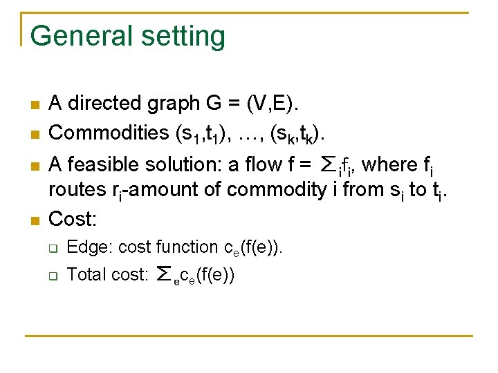
General setting n n A directed graph G = (V, E). Commodities (s 1, t 1), …, (sk, tk). A feasible solution: a flow f = ∑ifi, where fi routes ri-amount of commodity i from si to ti. Cost: q Edge: cost function ce(f(e)). q Total cost: ∑ece(f(e))

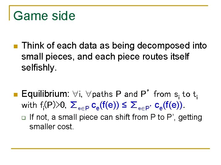
Game side n n Think of each data as being decomposed into small pieces, and each piece routes itselfishly. Equilibrium: i, paths P and P’ from si to ti with fi(P)>0, ∑e P ce(f(e)) ≤ ∑e P’ ce(f(e)). q If not, a small piece can shift from P to P’, getting smaller cost.

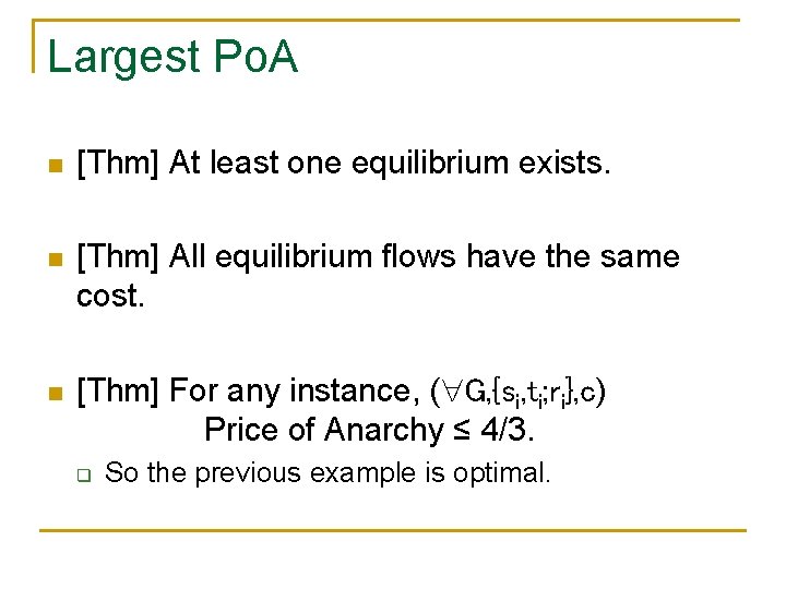
Largest Po. A n [Thm] At least one equilibrium exists. n [Thm] All equilibrium flows have the same cost. n [Thm] For any instance, ( G, {si, ti; ri}, c) Price of Anarchy ≤ 4/3. q So the previous example is optimal.

Part III. Game theory applied to computer science

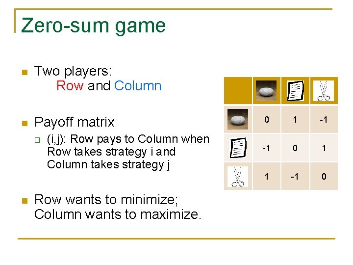
Zero-sum game n Two players: Row and Column n Payoff matrix q n (i, j): Row pays to Column when Row takes strategy i and Column takes strategy j Row wants to minimize; Column wants to maximize. 0 1 -1 -1 0 1 1 -1 0

Minimax theorem n 0 1 -1 -1 0 1 1 -1 0

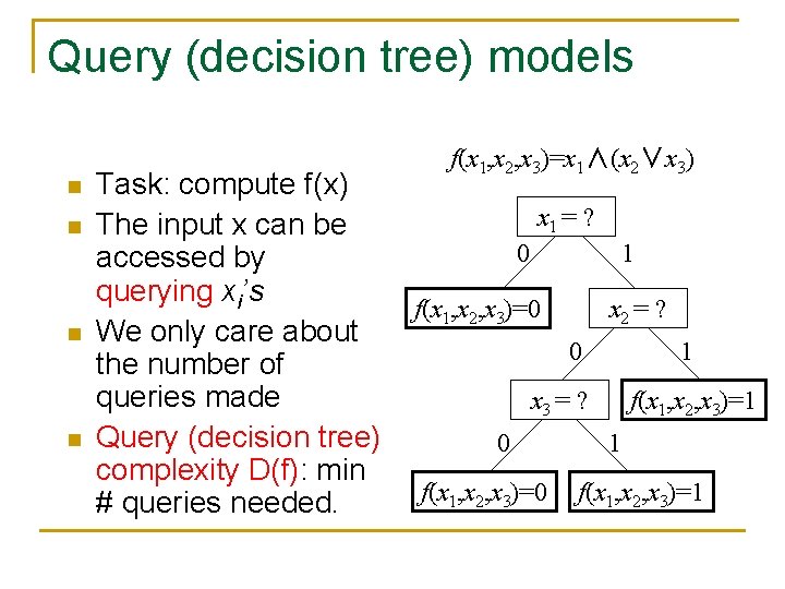
Query (decision tree) models n n f(x 1, x 2, x 3)=x 1∧(x 2∨x 3) Task: compute f(x) x 1 = ? The input x can be 0 1 accessed by querying xi’s f(x 1, x 2, x 3)=0 x 2 = ? We only care about 0 1 the number of queries made x 3 = ? f(x 1, x 2, x 3)=1 Query (decision tree) 0 1 complexity D(f): min f(x 1, x 2, x 3)=0 f(x 1, x 2, x 3)=1 # queries needed.

Randomized/Quantum query models n Randomized query model: q q We can toss a coin to decide the next query. R(f): randomized query complexity. n While D(f) is relatively easy to lower bound, R(f) is much harder. n Yao: Let algorithms and adversaries play a game!

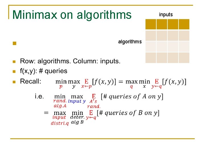
Minimax on algorithms inputs

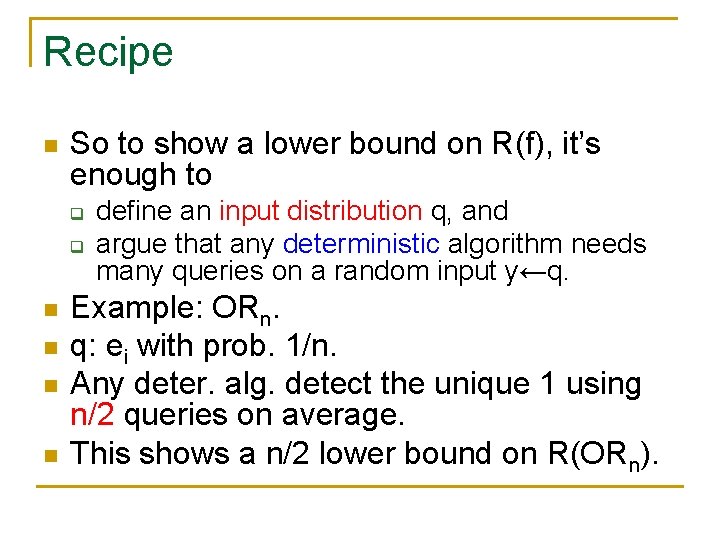
Recipe n So to show a lower bound on R(f), it’s enough to q q n n define an input distribution q, and argue that any deterministic algorithm needs many queries on a random input y←q. Example: ORn. q: ei with prob. 1/n. Any deter. alg. detect the unique 1 using n/2 queries on average. This shows a n/2 lower bound on R(ORn).