Shengyu Zhang The Chinese University of Hong Kong

Shengyu Zhang The Chinese University of Hong Kong

Why we are here? n Understanding the power of quantum q q q n Computation: quantum algorithms/complexity Communication: quantum info. theory … This work: game theory

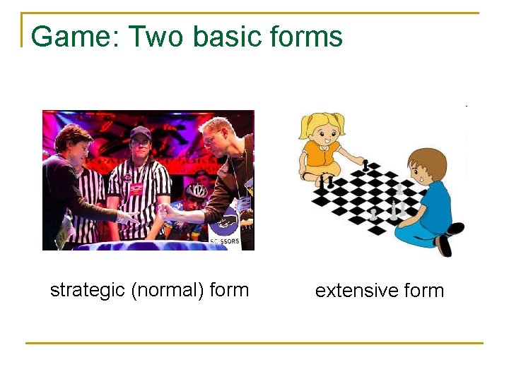
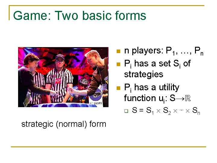
Game: Two basic forms strategic (normal) form extensive form

Game: Two basic forms n n players: P 1, …, Pn Pi has a set Si of strategies Pi has a utility function ui: S→ℝ q strategic (normal) form S = S 1 S 2 ⋯ Sn

Nash equilibrium n Nash equilibrium: each player has adopted an optimal strategy, provided that others keep their strategies unchanged

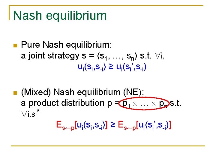
Nash equilibrium n Pure Nash equilibrium: a joint strategy s = (s 1, …, sn) s. t. i, ui(si, s-i) ≥ ui(si’, s-i) n (Mixed) Nash equilibrium (NE): a product distribution p = p 1 … pn s. t. i, si’ Es←p[ui(si, s-i)] ≥ Es←p[ui(si’, s-i)]

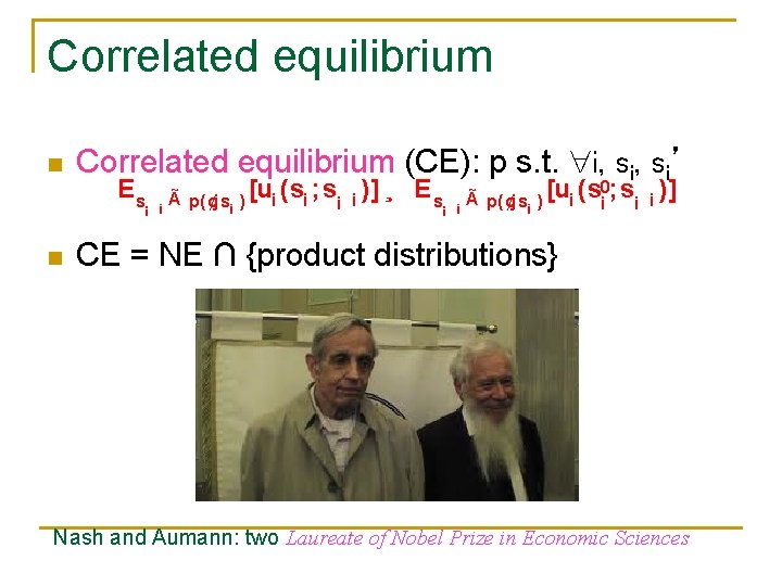
Correlated equilibrium n Correlated equilibrium (CE): p s. t. i, si’ Es ¡ n [ui (si ; s¡ i )] Ã ¢ p( js ) i i ¸ Es ¡ [ui (s 0 i; s¡ i )] Ã ¢ p( js ) i i CE = NE ∩ {product distributions} Nash and Aumann: two Laureate of Nobel Prize in Economic Sciences

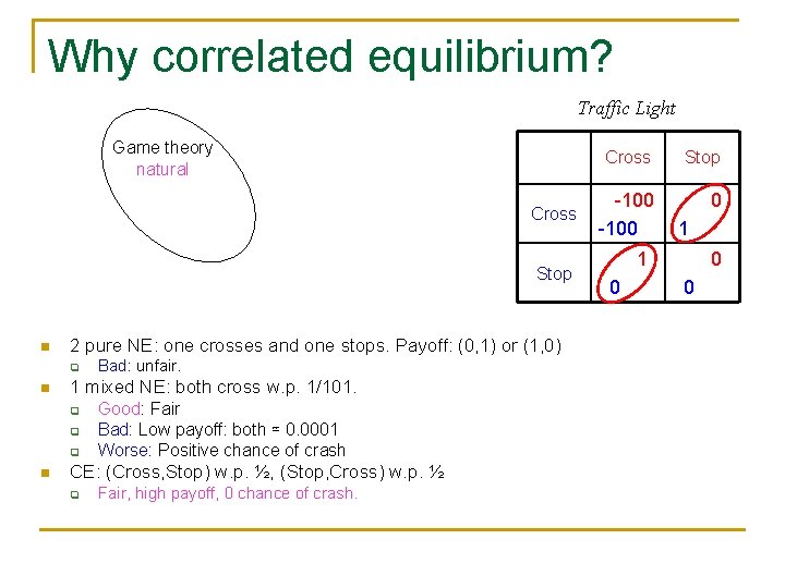
Why correlated equilibrium? Traffic Light Game theory natural Cross Stop n 2 pure NE: one crosses and one stops. Payoff: (0, 1) or (1, 0) q n 1 mixed NE: both cross w. p. 1/101. q q q n Bad: unfair. Good: Fair Bad: Low payoff: both ≃ 0. 0001 Worse: Positive chance of crash CE: (Cross, Stop) w. p. ½, (Stop, Cross) w. p. ½ q Fair, high payoff, 0 chance of crash. Cross Stop -100 0 1 1 0 0 0

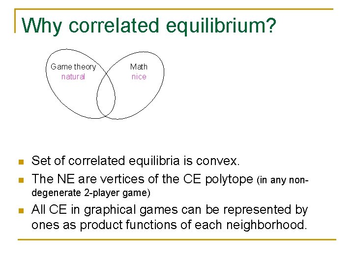
Why correlated equilibrium? Game theory natural n n Math nice Set of correlated equilibria is convex. The NE are vertices of the CE polytope (in any nondegenerate 2 -player game) n All CE in graphical games can be represented by ones as product functions of each neighborhood.

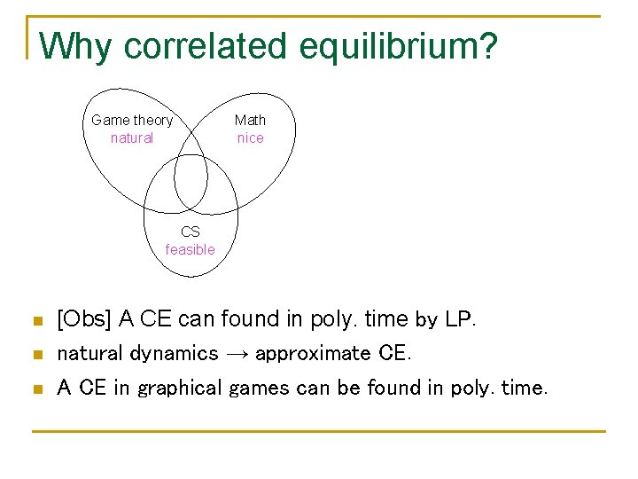
Why correlated equilibrium? Game theory natural Math nice CS feasible n n n [Obs] A CE can found in poly. time by LP. natural dynamics → approximate CE. A CE in graphical games can be found in poly. time.

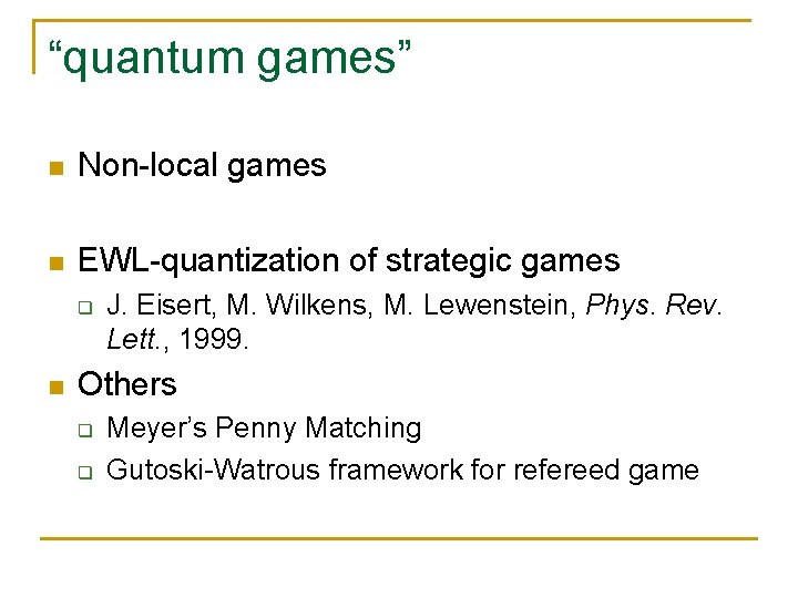
“quantum games” n Non-local games n EWL-quantization of strategic games q n J. Eisert, M. Wilkens, M. Lewenstein, Phys. Rev. Lett. , 1999. Others q q Meyer’s Penny Matching Gutoski-Watrous framework for refereed game

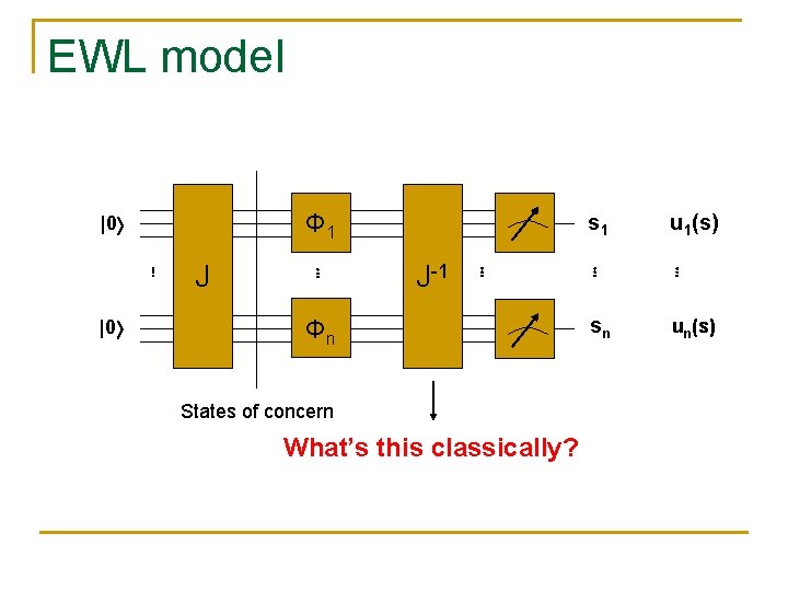
EWL model Φ 1 |0 ⋮ |0 J ⋮ J-1 ⋮ Φn States of concern What’s this classically? s 1 u 1(s) ⋮ ⋮ sn un(s)

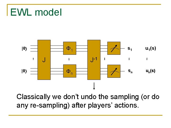
EWL model Φ 1 |0 ⋮ |0 J ⋮ Φn J-1 ⋮ s 1 u 1(s) ⋮ ⋮ sn un(s) Classically we don’t undo the sampling (or do any re-sampling) after players’ actions.

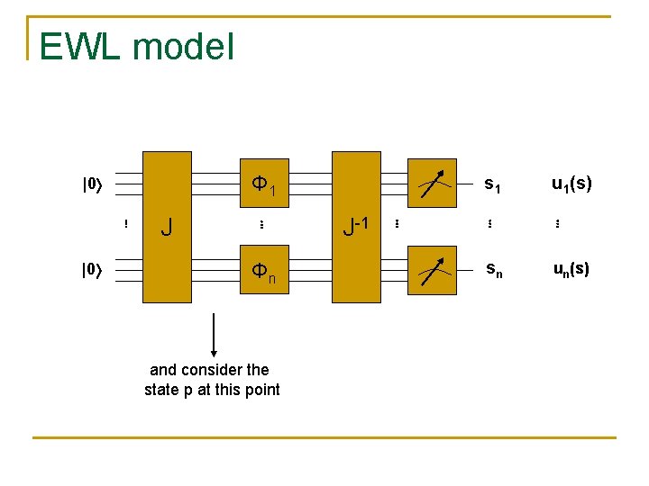
EWL model Φ 1 |0 ⋮ |0 J ⋮ Φn and consider the state p at this point J-1 ⋮ s 1 u 1(s) ⋮ ⋮ sn un(s)

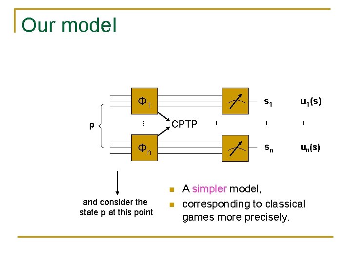
Our model Φ 1 ρ ⋮ CPTP Φn n and consider the state p at this point n ⋮ s 1 u 1(s) ⋮ ⋮ sn un(s) A simpler model, corresponding to classical games more precisely.

Other than the model n Main differences than previous work in quantum strategic games: n We consider general games of growing sizes. q n Previous: specific games, usually 2*2 or 3*3 We study quantitative questions. q q Previous work: advantages exist? Ours: How much can it be?

n Central question: How much “advantage” can playing quantum provide? n Measure 1: Increase of payoff Measure 2: Hardness of generation n

First measure: increase of payoff n We will define natural correspondences between classical distributions and quantum states. n And examine how well the equilibrium property is preserved.

Quantum equilibrium quantum classical p→ s C 1 s 1’ ⋮ ⋮ sn’ Cn u 1(s’) ⋮ un(s’) Φ 1 ρ ⋮ ⋮ Φn s 1 u 1(s) ⋮ ⋮ sn un(s) classical equilibrium: quantum equilibrium: No player wants to do anything to the assigned strategy si, if others do nothing on their parts - p = p 1 … pn: Nash equilibrium - general p: correlated equilibrium No player wants to do anything to the assigned strategy ρ|Hi, if others do nothing on their parts - ρ = ρ1 … ρn: quantum Nash equilibrium - general ρ: quantum correlated equilibrium

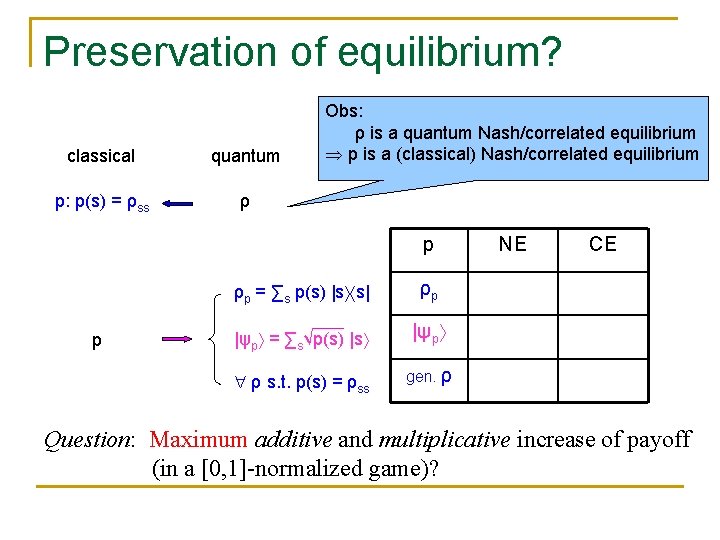
Correspondence of classical and quantum states quantum classical p→s C 1 s 1’ Cn sn’ ⋮ p: p(s) = ρss ⋮ Φ 1 ρ ⋮ ⋮ Φn s 1 ⋮ sn ρ (measure in comp. basis) p: distri. on S ρp = ∑s p(s) |s s| (classical mixture) |ψp = ∑s√p(s) |s (quantum superposition) ρ s. t. p(s) = ρss (general class)

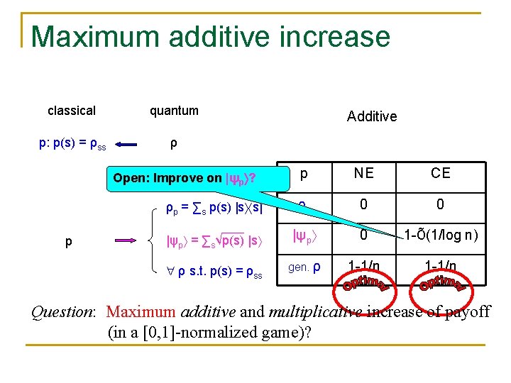
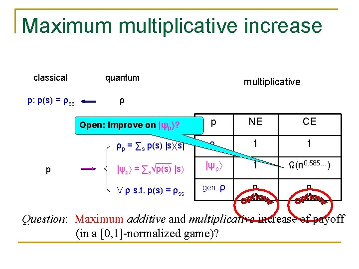
Preservation of equilibrium? classical quantum p: p(s) = ρss ρ Obs: ρ is a quantum Nash/correlated equilibrium p is a (classical) Nash/correlated equilibrium p p ρp = ∑s p(s) |s s| ρp |ψp = ∑s√p(s) |s |ψp ρ s. t. p(s) = ρss NE CE gen. ρ Question: Maximum additive and multiplicative increase of payoff (in a [0, 1]-normalized game)?

Maximum additive increase classical quantum p: p(s) = ρss ρ p NE CE ρp = ∑s p(s) |s s| ρp 0 0 |ψp = ∑s√p(s) |s |ψp 0 1 -Õ(1/log n) gen. ρ 1 -1/n Open: Improve on |ψp ? p Additive ρ s. t. p(s) = ρss Question: Maximum additive and multiplicative increase of payoff (in a [0, 1]-normalized game)?

Maximum multiplicative increase classical quantum p: p(s) = ρss ρ p NE CE ρp = ∑s p(s) |s s| ρp 1 1 |ψp = ∑s√p(s) |s |ψp 1 Ω(n 0. 585…) gen. ρ n n Open: Improve on |ψp ? p multiplicative ρ s. t. p(s) = ρss Question: Maximum additive and multiplicative increase of payoff (in a [0, 1]-normalized game)?

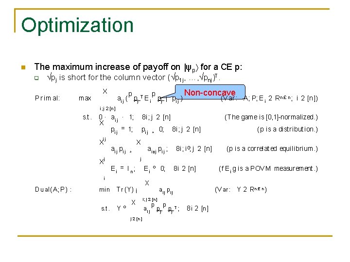
Optimization n The maximum increase of payoff on |ψp for a CE p: q √pj is short for the column vector (√p 1 j, …, √pnj)T. P r im al: max Non-concave p p ai j ( pj T E i pj ¡ pi j ) (V ar : A; P; E i 2 Rn £ n ; i 2 [n]) X i ; j 2 [n ] s. t. 8 i ; j 2 [n] 0 · ai j · 1; X pi j = 1; ij X min s. t. ai 0 j pi j ; 8 i ; i 0; j 2 [n] (p is a dist ribut ion. ) (p is a correlat ed equilibrium. ) j Ei = I n ; i D ual (A ; P ) : 8 i ; j 2 [n] pi j ¸ 0; X ai j pi j ¸ (T he game is [0, 1]-normalized. ) T r (Y ) ¡ Y º X j 2 [n ] E i º 0; X ai j pi j i ; j 2 [n ] ai j 8 i 2 [n] p pj T ; (f E i g is a POVM measurement. ) (V ar : Y 2 Rn £ n ) 8 i 2 [n]

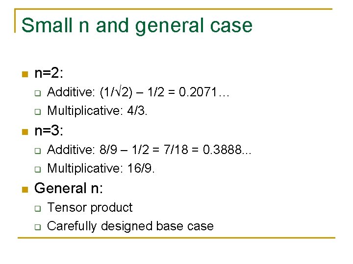
Small n and general case n n=2: q q n n=3: q q n Additive: (1/√ 2) – 1/2 = 0. 2071… Multiplicative: 4/3. Additive: 8/9 – 1/2 = 7/18 = 0. 3888. . . Multiplicative: 16/9. General n: q q Tensor product Carefully designed base case

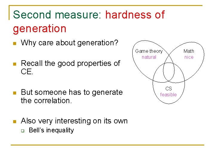
Second measure: hardness of generation n n Why care about generation? Recall the good properties of CE. n But someone has to generate the correlation. n Also very interesting on its own q Bell’s inequality Game theory natural CS feasible Math nice

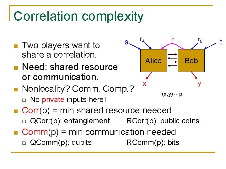
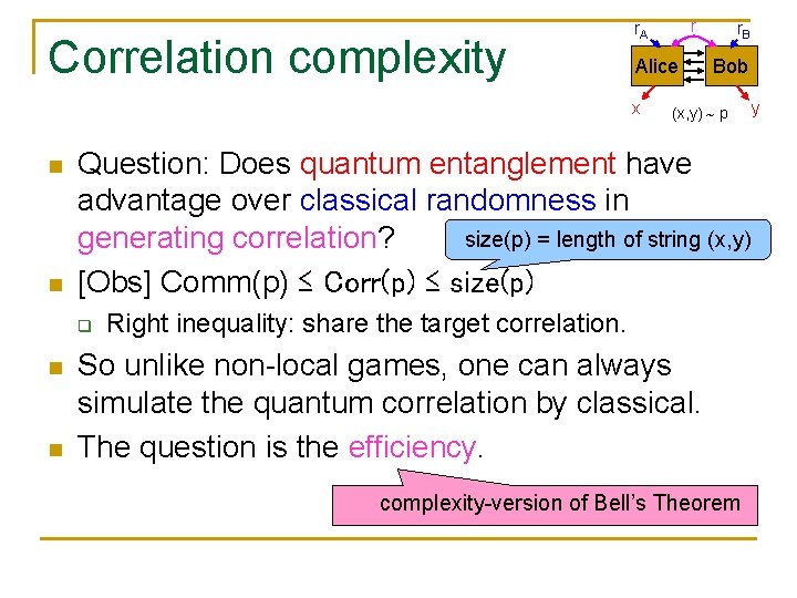
Correlation complexity n n n Two players want to share a correlation. Nonlocality? Comm. Comp. ? r r. B Bob x y (x, y) p Corr(p) = min shared resource needed q n No private inputs here! r. A Alice Need: shared resource or communication. q n s QCorr(p): entanglement RCorr(p): public coins Comm(p) = min communication needed q QComm(p): qubits RComm(p): bits t

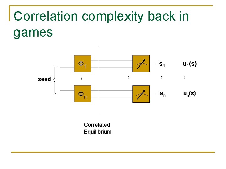
Correlation complexity back in games Φ 1 seed ⋮ ⋮ Φn Correlated Equilibrium s 1 u 1(s) ⋮ ⋮ sn un(s)

Correlation complexity Alice x n n n r. B Bob (x, y) p Question: Does quantum entanglement have advantage over classical randomness in size(p) = length of string (x, y) generating correlation? [Obs] Comm(p) ≤ Corr(p) ≤ size(p) q n r r. A Right inequality: share the target correlation. So unlike non-local games, one can always simulate the quantum correlation by classical. The question is the efficiency. complexity-version of Bell’s Theorem y

Separation n [Conj] A random with [Thm] p=(X, Y) of size n, s. t. QCorr(p) = 1, RComm(p) ≥ log(n). n

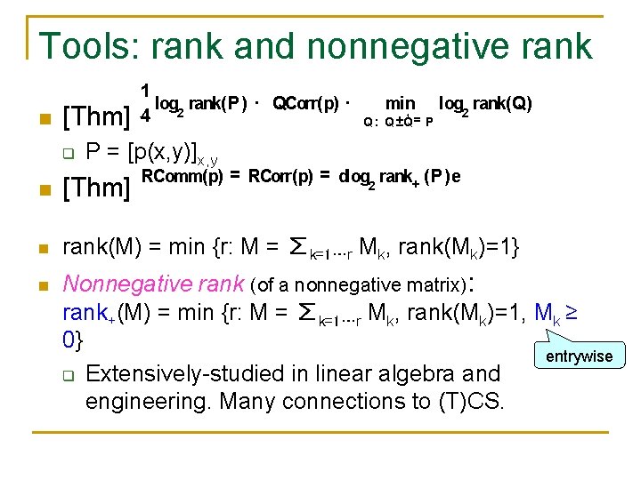
Tools: rank and nonnegative rank n [Thm] q 1 log 2 rank(P ) · QCorr(p) · 4 min ¹=P Q : Q ±Q log 2 rank(Q) P = [p(x, y)]x, y RComm(p) = RCorr(p) = dlog 2 rank+ (P )e n [Thm] n rank(M) = min {r: M = ∑k=1…r Mk, rank(Mk)=1} n Nonnegative rank (of a nonnegative matrix): rank+(M) = min {r: M = ∑k=1…r Mk, rank(Mk)=1, Mk ≥ 0} entrywise q Extensively-studied in linear algebra and engineering. Many connections to (T)CS.

Explicit instances n Euclidean Distance Matrix (EDM): Q(i, j) = ci – cj where c 1, …, c. N ℝ. q q q rank(Q) = 2. [Thm, BL 09] rank+(Q∘Q) ≥ log 2 N [Conj, BL 09] rank+(Q∘Q) = N. (Even existing one Q implies 1 vs. n separation, the strongest possible)

Conclusion n Model: natural, simple, rich q n Non-convex programming; rank+; comm. comp. Next directions: q q Improve the bounds (in both measures) Efficient testing of QNE/QCE? QCE ← natural quantum dynamics? Approximate Correlation complexity n q [Shi-Z] p: QCorrε(p) = O(log n), RCommε(p) = Ω(√n) Characterize QCorr? n Mutual info? No! p: Ip = O(n-1/4), QCorr(p) = Θ(log n)

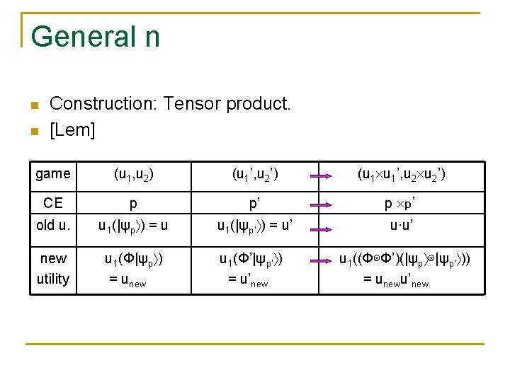
General n n n Construction: Tensor product. [Lem] game (u 1, u 2) (u 1’, u 2’) (u 1 u 1’, u 2’) CE p p’ old u. u 1(|ψp ) = u u 1(|ψp’ ) = u’ u∙u’ new utility u 1(Φ|ψp ) = unew u 1(Φ’|ψp’ ) = u’new u 1((Φ⊗Φ’)(|ψp ⊗|ψp’ )) = unewu’new

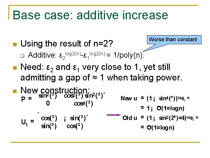
Base case: additive increase n Using the result of n=2? q n n Worse than constant Additive: ε 2 log 2(n)-ε 1 log 2(n) = 1/poly(n). Need: ε 2 and ε 1 very close to 1, yet still admitting a gap of ≈ 1 when taking power. ¸ New· construction: 2 2 2 sin (²) P= 0 · cos(²) = U 1 sin(²) cos (²) sin (²) cos 4 (²) ¸ ¡ sin(²) cos(²) New u = (1 ¡ sin 4 (²)) log 2 n ~ = 1 ¡ O(1=logn) Old u = (1 ¡ sin 2 (2²)=4) log 2 n ~ = O(1=logn)