Lecture 13 Inner Product Space Linear Transformation Last

Lecture 13 Inner Product Space & Linear Transformation Last Time - Orthonormal Bases: Gram-Schmidt Process - Mathematical Models and Least Square Analysis - Inner Product Space Applications Elementary Linear Algebra R. Larsen et al. (5 Edition) TKUEE翁慶昌-NTUEE SCC_12_2007

Lecture 12: Inner Product Spaces & L. T. Today n Mathematical Models and Least Square Analysis n Inner Product Space Applications n Introduction to Linear Transformations Reading Assignment: Secs 5. 4, 5. 5, 6. 1, 6. 2 Next Time n The Kernel and Range of a Linear Transformation n Matrices for Linear Transformations n Transition Matrix and Similarity Reading Assignment: Secs 6. 2 -6. 4 13 - 2

What Have You Actually Learned about Projection So Far? 13 - 3

5. 4 Mathematical Models and Least Squares Analysis n Orthogonal complement of W: Let W be a subspace of an inner product space V. (a) A vector u in V is said to orthogonal to W, if u is orthogonal to every vector in W. (b) The set of all vectors in V that are orthogonal to W is called the orthogonal complement of W. (read “ § Notes: 13 - 4 perp”)

n Direct sum: Let and be two subspaces of . If each vector can be uniquely written as a sum of a vector n and a vector from direct sum of and , , then , and you can write from is the. Thm 5. 13: (Properties of orthogonal subspaces) Let W be a subspace of Rn. Then the following properties are true. (1) (2) (3) 13 - 5

n Find by the other method: 13 - 6

n Thm 5. 16: (Fundamental subspaces of a matrix) If A is an m×n matrix, then (1) (2) (3) (4) 13 - 7

n Ex 6: (Fundamental subspaces) Find the four fundamental subspaces of the matrix. (reduced row-echelon form) Sol: 13 - 8

n Check: 13 - 9

n Ex 3: Let W is a subspace of R 4 and . (a) Find a basis for W (b) Find a basis for the orthogonal complement of W. Sol: (reduced row-echelon form) 13 - 10

is a basis for W n Notes: 13 - 11

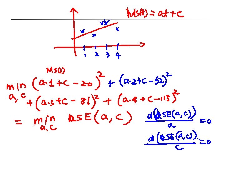
Least Squares Problem n Least squares problem: (A system of linear equations) (1) When the system is consistent, we can use the Gaussian elimination with back-substitution to solve for x (2) When the system is consistent, how to find the “best possible” solution of the system. That is, the value of x for which the difference between Ax and b is small. 13 - 12

n Least squares solution: Given a system Ax = b of m linear equations in n unknowns, the least squares problem is to find a vector x in Rn that minimizes with respect to the Euclidean inner product on Rn. Such a vector is called a least squares solution of Ax = b. 13 - 13

(the normal system associated with Ax = b) 13 - 14

n Note: The problem of finding the least squares solution of is equal to he problem of finding an exact solution of the associated normal system n . Thm: For any linear system , the associated normal system is consistent, and all solutions of the normal system are least squares solution of Ax = b. Moreover, if W is the column space of A, and x is any least squares solution of Ax = b, then the orthogonal projection of b on W is 13 - 15

n Thm: If A is an m×n matrix with linearly independent column vectors, then for every m× 1 matrix b, the linear system Ax = b has a unique least squares solution. This solution is given by Moreover, if W is the column space of A, then the orthogonal projection of b on W is 13 - 16

n Ex 7: (Solving the normal equations) Find the least squares solution of the following system and find the orthogonal projection of b on the column space of A. 13 - 17

n Sol: the associated normal system 13 - 18

the least squares solution of Ax = b the orthogonal projection of b on the column space of A 13 - 19

Keywords in Section 5. 4: n orthogonal to W: 正交於W n orthogonal complement: 正交補集 n direct sum: 直和 n projection onto a subspace: 在子空間的投影 n fundamental subspaces: 基本子空間 n least squares problem: 最小平方問題 n normal equations: 一般方程式 13 - 20

Application: Cross Product Cross product (vector product) of two vectors 向量(vector) 方向: use right-hand rule The cross product is not commutative: The cross product is distributive: 13 - 23

Application: Cross Product Parallelogram representation of the vector product y Bsinθ Area θ x 13 - 24

向量之三重純量積 Triple Scalar product 純量(scalar) The dot and the cross may be interchanged : 13 - 25

向量之三重純量積 Parallelepiped representation of triple scalar product Volume of parallelepiped defined by z y x 13 - 26 , , and

Fourier Approximation 13 - 27

Fourier Approximation n n The Fourier series transforms a given periodic function into a superposition of sine and cosine waves The following equations are used 13 - 28

Today n Mathematical Models and Least Square Analysis (Cont. ) n Inner Product Space Applications n Introduction to Linear Transformations n The Kernel and Range of a Linear Transformation 12 - 29

6. 1 Introduction to Linear Transformations n Function T that maps a vector space V into a vector space W: V: the domain of T W: the codomain of T 13 - 30

n Image of v under T: If v is in V and w is in W such that Then w is called the image of v under T. n n the range of T: The set of all images of vectors in V. the preimage of w: The set of all v in V such that T(v)=w. 13 - 31

n Ex 1: (A function from R 2 into R 2 ) (a) Find the image of v=(-1, 2). (b) Find the preimage of w=(-1, 11) Sol: Thus {(3, 4)} is the preimage of w=(-1, 11). 13 - 32

n Linear Transformation (L. T. ): 13 - 31

n Notes: (1) A linear transformation is said to be operation preserving. Addition in V Addition in W Scalar multiplication in V Scalar multiplication in W (2) A linear transformation from a vector space into itself is called a linear operator. 13 - 34

n Ex 2: (Verifying a linear transformation T from R 2 into R 2) Pf: 13 - 35

Therefore, T is a linear transformation. 13 - 36

n Ex 3: (Functions that are not linear transformations) 13 - 37

n Notes: Two uses of the term “linear”. (1) is called a linear function because its graph is a line. (2) is not a linear transformation from a vector space R into R because it preserves neither vector addition nor scalar multiplication. 13 - 38

n Zero transformation: n Identity transformation: n Thm 6. 1: (Properties of linear transformations) 13 - 39

n Ex 4: (Linear transformations and bases) Let be a linear transformation such that Find T(2, 3, -2). Sol: (T is a L. T. ) 13 - 40

n Ex 5: (A linear transformation defined by a matrix) The function is defined as Sol: (vector addition) (scalar multiplication) 13 - 41

n Thm 6. 2: (The linear transformation given by a matrix) Let A be an m n matrix. The function T defined by is a linear transformation from Rn into Rm. n Note: 13 - 42

n Ex 7: (Rotation in the plane) Show that the L. T. given by the matrix has the property that it rotates every vector in R 2 counterclockwise about the origin through the angle . Sol: (polar coordinates) r： the length of v ：the angle from the positive x-axis counterclockwise to the vector v 13 - 43

r：the length of T(v) + ：the angle from the positive x-axis counterclockwise to the vector T(v) Thus, T(v) is the vector that results from rotating the vector v counterclockwise through the angle . 13 - 44

n Ex 8: (A projection in R 3) The linear transformation is given by is called a projection in R 3. 13 - 45

n Ex 9: (A linear transformation from Mm n into Mn m ) Show that T is a linear transformation. Sol: Therefore, T is a linear transformation from Mm n into Mn m. 13 - 46

Keywords in Section 6. 1: n function: 函數 n domain: 論域 n codomain: 對應論域 n image of v under T: 在T映射下v的像 n range of T: T的值域 n preimage of w: w的反像 n linear transformation: 線性轉換 n linear operator: 線性運算子 n zero transformation: 零轉換 n identity transformation: 相等轉換 13 - 47

Today n Mathematical Models and Least Square Analysis (Cont. ) n Inner Product Space Applications n Introduction to Linear Transformations n The Kernel and Range of a Linear Transformation 13 - 48

6. 2 The Kernel and Range of a Linear Transformation n Kernel of a linear transformation T: Let be a linear transformation Then the set of all vectors v in V that satisfy called the kernel of T and is denoted by ker(T). n Ex 1: (Finding the kernel of a linear transformation) Sol: 13 - 49 is

n Ex 2: (The kernel of the zero and identity transformations) (a) T(v)=0 (the zero transformation (b) T(v)=v (the identity transformation n ) ) Ex 3: (Finding the kernel of a linear transformation) Sol: 13 - 50