Lecture 03 Aliasing and Neighborhood of Pixels Aliasing

Lecture # 03 Aliasing and Neighborhood of Pixels

Aliasing and Moire Patterns Functions whose area under the curve is finite can be represented in terms of sines and cosines of various frequencies. The sine/cosine component with the highest frequency determines the highest "frequency content" of the function. Suppose that this highest frequency is finite and that the function is of unlimited duration (these functions are called band-limited functions). Then, the Shannon sampling theorem tells us that, if the function is sampled at a rate equal to or greater than twice its highest frequency, it is possible to recover completely the original function from its samples. If the function is undersampled, then a phenomenon called aliasing corrupts the sampled image. The corruption is in the form of additional frequency components being introduced into the sampled function. These are called aliased frequencies. Note that the sampling rate in images is the number of samples taken (in both spatial directions) per unit distance.

How Aliasing Can Be Reduced? It is impossible to satisfy the sampling theorem in practice. We can only work with sampled data that are finite in duration. We can model the process of converting a function of unlimited duration into a function of finite duration simply by multiplying the unlimited function by a "gating function" that is valued 1 for some interval and 0 elsewhere. Unfortunately, this function itself has frequency components that extend to infinity. Thus, the very act of limiting the duration of a band-limited function causes it to cease being band limited, which causes it to violate the key condition of the sampling theorem. The principal approach for reducing the aliasing effects on an image is to reduce its high-frequency components by blurring the image prior to sampling. However, aliasing is always present in a sampled image. The effect of aliased frequencies can be seen under the right conditions in the form of so called Moire patterns.

Moire Patterns Figure A
 There is one special case of")
How Aliasing Can Be Reduced? (contd. . ) There is one special case of significant importance in which a function of infinite duration can be sampled over a finite interval without violating the sampling theorem. When a function is periodic, it may be sampled at a rate equal to or exceeding twice its highest frequency, and it is possible to recover the function from its samples provided that the sampling captures exactly an integer number of periods of the function.

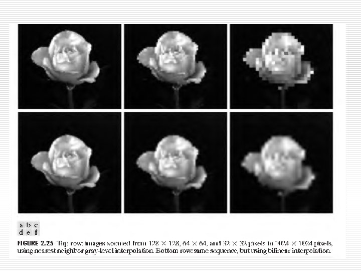
Zooming and Shrinking Digital Images This topic is related to image sampling and quantization because zooming may be viewed as over sampling, while shrinking may be viewed as under samp ling. Zooming requires two steps: 1. The creation of new pixel locations, 2. and the assignment of gray levels to those new locations. Let us start with a simple example. Suppose that we have an image of size 500 X 500 pixels and we want to enlarge it 1. 5 times to 750 X 750 pixels. Conceptually, one of the easiest ways to visualize zooming is laying an imaginary 750 X 750 grid over the original image. Obviously, the spacing in the grid would be less than one pixel because we are fitting it over a smaller image. In order to perform gray-level assignment for any point in the overlay, we look for the closest pixel in the original image and assign its gray level to the new pixel in the grid. When we are done with all points in the overlay grid, we simply expand it to the original specified size to obtain the zoomed image. This method of gray-level assignment is called nearest neighbor interpolation.

Pixel Replication & Bilinear interpolation Pixel replication is a special case of nearest neighbor interpolation. Pixel replication is applicable when we want to increase the size of an image an integer number of times. For instance, to double the size of an image, we can duplicate each column. This doubles the image size in the horizontal direction. Then, we duplicate each row of the enlarged image to double the size in the vertical direction. The same procedure is used to enlarge the image by any integer number of times (triple, quadruple, and so on). Duplication is just done the required number of times to achieve the desired size. The gray-level assignment of each pixel is predetermined by the fact that new locations are exact duplicates of old locations. Although nearest neighbor interpolation is fast, it has the undesirable feature that it produces a checkerboard effect that is particularly objectionable at high factors of magnification. A slightly more sophisticated way of accomplishing gray-level assignments is bilinear interpolation using the four nearest neighbors of a point.

Image Shrinking Image shrinking is done in a similar manner as just described for zooming. The equivalent process of pixel replication is row-column deletion. For example, to shrink an image by one-half, we delete every other row and column. We can use the zooming grid analogy to visualize the concept of shrinking by a noninteger factor, except that we now expand the grid to fit over the original image, do gray-level nearest neighbor or bilinear interpolation, and then shrink the grid back to its original specified size. To reduce possible aliasing effects, it is a good idea to blur an image slightly before shrinking it. Extra computational burden seldom is justifiable for general-purpose digital image zooming and shrinking, where bilinear interpolation generally is the method of choice.

Neighborhood of Pixels: o A Digital Image, comprises of a 2 D matrix and every element is called as Pixel. o The Image is denoted by f(x, y) and any pixel can be denoted by small letter, say p, q … o Every Pixel has some Neighbors located around it. o Different types of neighbors include: n n n 4 Neighbors D Neighbors 8 Neighbors 10

Neighborhood of Pixels: o 4 Neighbors n A pixel ’p’ located at coordinate value (x, y) has 4 neighbors, which are adjacent to ‘p’. n The coordinate values can be determined as: n (x+1, y) n (x-1, y) n (x, y+1) n (x, y-1) (x, y+1) (x-1, y) p (x, y) (x+1, y) (x, y-1) 4 Neighbors are denoted by N 4(p) 11

Neighborhood of Pixels: o D Neighbors n A pixel ’p’ located at coordinate value (x, y) has D neighbors, which are located in Diagonal of ‘p’. n The coordinate values can be determined as: n n (x+1, y+1) (x+1, y-1) (x-1, y+1) (x-1, y-1) (x-1, y+1) (x+1, y+1) p (x, y) (x-1, y-1) D Neighbors are denoted by ND(p) (x+1, y-1) 12

Neighborhood of Pixels: o 8 Neighbors n A pixel ’p’ located at coordinate value (x, y) has 8 neighbors, which are combination of 4 and D Neighbors. (x-1, y+1) (x-1, y-1) (x, y+1) p(x, y) (x, y-1) (x+1, y+1) (x+1, y-1) 8 Neighbors are denoted by N 8(p) 13

Neighborhood of Pixels: o Some of the Neighbors can be outside the Image, if the pixel ‘p’ is located at the border of the Image. 2 3 5 1 9 6 4 8 7 o If “ 9” is considered as pixel ‘p’ then: N 4(p)= {1, 3, 8, 6} o If “ 1” is considered as pixel ‘p’ then: N 4(p)= {2, 4, 9} (one Neighbor is not available) 14

Connectivity: o Connectivity between pixels is an important concept used in establishing boundaries of objects and components of regions in an image. o As we can identify different objects in Image depending upon the Intensity values of Pixels. o So all Pixels comprising an object would have Same /Close values. 15

Connectivity: o To establish whether two pixels are connected, it must be determined n If they are adjacent in some sense (say, if they are 4 neighbors). and n If their grey levels satisfy a specified criterion of similarity. 16
 can be defined by defining a")
Connectivity: o The specified Criteria (Intensity Range ) can be defined by defining a set ‘V’ at start. n For V={2} o Only those Pixel can be connected which have value =2 n For V={1, 2} o Only those Pixel can be connected which have value =1 or 2. 17
: o 4 Connectivity: o Two pixels p and q with values from")
Connectivity (Adjacency): o 4 Connectivity: o Two pixels p and q with values from V are 4 - connected if q is in the set N 4 (p). o 8 Connectivity: o Two pixels p and q with values from V are 8 - connected if q is in the set N 8 (p). o M-Connectivity (Mixed Connectivity): o Two pixels p and q with values from V are m- connected if: • q is in N 4 (p), OR • q is in ND (p) AND the set N 4 (p) ∩ N 4 (q) is empty. 18
: Ø Mixed adjacency is a modification of 8 -adjacency. It is")
M-Connectivity (Mixed Connectivity): Ø Mixed adjacency is a modification of 8 -adjacency. It is introduced to eliminate the ambiguities that often arise when 8 -adjacency is used. 19

Example of Connectivity: 0 1 1 0 0 0 1 20

4 - connectivity: 0 1 1 0 0 0 1 21

8 - connectivity: 0 1 1 0 0 0 1 22

M-connectivity: 0 1 1 0 0 0 1 Duplicate Link removed. 23

Example 2 o Consider two image subsets, S 1 & S 2 shown in the following figure. For V={1} , determine whether these two subsets are (a)4 adjacent (b) 8 adjacent (c) m-adjacent 24
. Let p and q be as shown in the Fig. Then, (a)")
Solution(Example 2). Let p and q be as shown in the Fig. Then, (a) S 1 and S 2 are not 4 connected because q is not in the set N 4(p). (b) S 1 and S 2 are 8 connected because q is in the set N 8(p). (c) S 1 and S 2 are mconnected because (i) q is in ND(p), and (ii) the set N 4(p) N 4(q) is empty. 25
 Let V={0, 1} and")
Example 3 o Consider the image segment given below. (a) Let V={0, 1} and compute the lengths of the shortest 4, 8 and m-path between p & q. If the particular path does not exist between these two points explain why. (b) Repeat for V={1, 2}. 3 1 2 1(q) 2 2 0 2 1 1 (P) 1 0 1 2 26
. (a) When V = {0, 1}; 4 path does not exist between")
Solution(Example 3). (a) When V = {0, 1}; 4 path does not exist between p and q because it is impossible to get from p to q by traveling along points that are both 4 adjacent and also have values from V. Figure (a) shows this condition; it is not possible to get to q. The shortest 8 path is shown in Fig. (b); its length is 4. The length of the shortest mpath (shown dashed) is 5. Both of these shortest paths are unique in this case. (b) One possibility for the shortest 4 path when V = {1, 2}; is shown in Fig. (c); its length is 6. It is easily verified that another 4 path of the same length exists between p and q. One possibility for the shortest 8 path (it is not unique) is shown in Fig. (d); its length is 4. The length of a shortest mpath (shown dashed) is 6. This path is not unique. Figures are shown on the next slide 27
4 path for V = {0, 1} (b)8 path(Solid Lines),")
Figures For Example 3 (a)4 path for V = {0, 1} (b)8 path(Solid Lines), m path(Dashed Lines) 28 (c) 4 path for V = {1, 2} (d) 8 path(Solid Lines), m path(Dashed Lines)

Example Task to do: v = {0} n 0 1 1 0 0 0 1 Solve this for 4 , 8 and m - Connectivity 29

Distance Measures: o If we have three pixels p, q & z, located in an Image at different positions with co-ordinates such as: p (x , y) , q (s , t) & z (u , v). o D is the distance function or metric if: 1. D ( p , q ) >= 0 2. 3. D(p, q) = D ( p , z ) <= ( D ( p , q ) = 0 iff p = q ). D(q, p), ( D ( p , q) + D ( q , z )). 30

Euclidian Distance: o Euclidean distance between p and q is given by: 2 2 1/2 DE( p , q ) = [ ( x - s) + ( y – t ) ] o For this distance measure , the pixel (s) having a D E distance less than or equal to some value r from (x , y) are the points contained in a disk of radius r centered at (x , y). 31

D 4 Distance : o It is also called as city-block distance and is defined between p and q as : D 4 ( p , q ) = o ( x-s ) + ( y-t ) For this distance measure, the pixel (s) having a D 4 distance from (x, y) less than or equal to some value r from a diamond centered at (x, y). 32

D 4 Distance : o All the pixels having D 4 distance less than or equal to 2, from the following contours of the constant distance: 2 2 1 0 1 2 2 o Diamond formed by Pixels around the center (x, y). o The pixel with D 4 = 1 are the neighbors of (x, y). 33
 between")
D 8 Distance: o The D 8 distance is also called (chessboard distance) between p and q is defined as: D 8 ( p , q ) = max ( ( x - s ) o , ( y-t) ) For this distance measure, the pixel (s) having a D 8 distance from (x, y) less than or equal to some value r, forms a SQUARE centered at (x, y). 34

D 8 Distance: o The pixel with D 8 distance <= 2 from (x, y) (the center point) from the following contours of constant distance: 2 2 2 1 1 1 2 2 1 0 1 2 2 1 1 1 2 2 2 o Square formed by Pixels around the center (x, y). o The pixel with D 8 = 1 are the 8 -neighbours of (x, y). 35
- Slides: 35