Digital Image Processing Digital Image Fundamentals Chapter 2

ﺑﺴﻤﻪﺗﻌﺎﻟﻲ Digital Image Processing Digital Image Fundamentals (Chapter 2) H. R. Pourreza

1. Introduction • In many image processing applications, the objective is to help a human observer perceive the visual information in an image. Therefore, it is important to understand the human visual system. • The human visual system consists mainly of the eye (image sensor or camera), optic nerve (transmission path), and brain (image information processing unit or computer). • It is one of the most sophisticated image processing and analysis systems. H. R. Pourreza

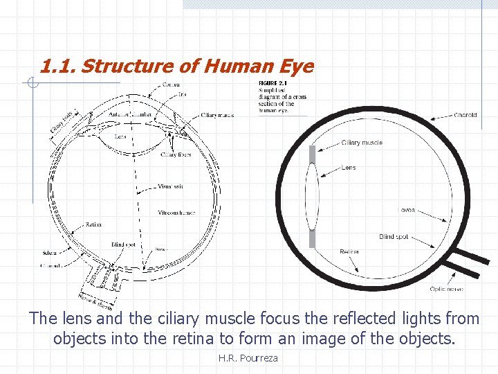
1. 1. Structure of Human Eye The lens and the ciliary muscle focus the reflected lights from objects into the retina to form an image of the objects. H. R. Pourreza

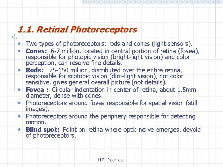
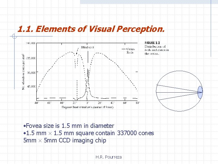
1. 1. Retinal Photoreceptors • Two types of photoreceptors: rods and cones (light sensors). • Cones: 6 -7 million, located in central portion of retina (fovea), • • • responsible for photopic vision (bright-light vision) and color perception, can resolve fine details. Rods: 75 -150 million, distributed over the entire retina, responsible for scotopic vision (dim-light vision), not color sensitive, gives general overall picture (not details). Fovea : Circular indentation in center of retina, about 1. 5 mm diameter, dense with cones. Photoreceptors around fovea responsible for spatial vision (still images). Photoreceptors around the periphery responsible for detecting motion. Blind spot: Point on retina where optic nerve emerges, devoid of photoreceptors. H. R. Pourreza

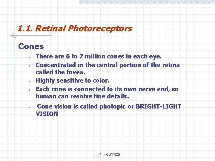
1. 1. Retinal Photoreceptors Cones • • • There are 6 to 7 million cones in each eye. Concentrated in the central portion of the retina called the fovea. Highly sensitive to color. Each cone is connected to its own nerve end, so human can resolve fine details. Cone vision is called photopic or BRIGHT-LIGHT VISION H. R. Pourreza

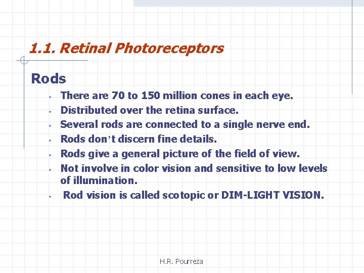
1. 1. Retinal Photoreceptors Rods • • There are 70 to 150 million cones in each eye. Distributed over the retina surface. Several rods are connected to a single nerve end. Rods don’t discern fine details. Rods give a general picture of the field of view. Not involve in color vision and sensitive to low levels of illumination. Rod vision is called scotopic or DIM-LIGHT VISION. H. R. Pourreza

1. 1. Elements of Visual Perception. • Fovea size is 1. 5 mm in diameter • 1. 5 mm square contain 337000 cones 5 mm CCD imaging chip H. R. Pourreza

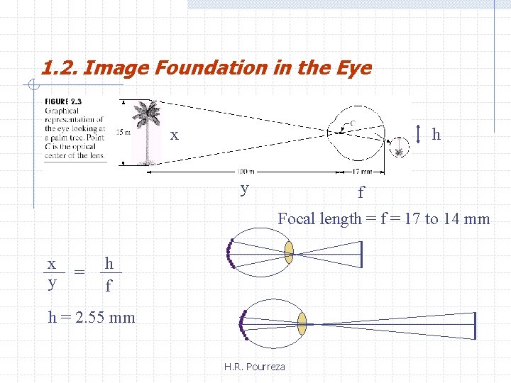
1. 2. Image Foundation in the Eye x h y f Focal length = f = 17 to 14 mm x y = h f h = 2. 55 mm H. R. Pourreza

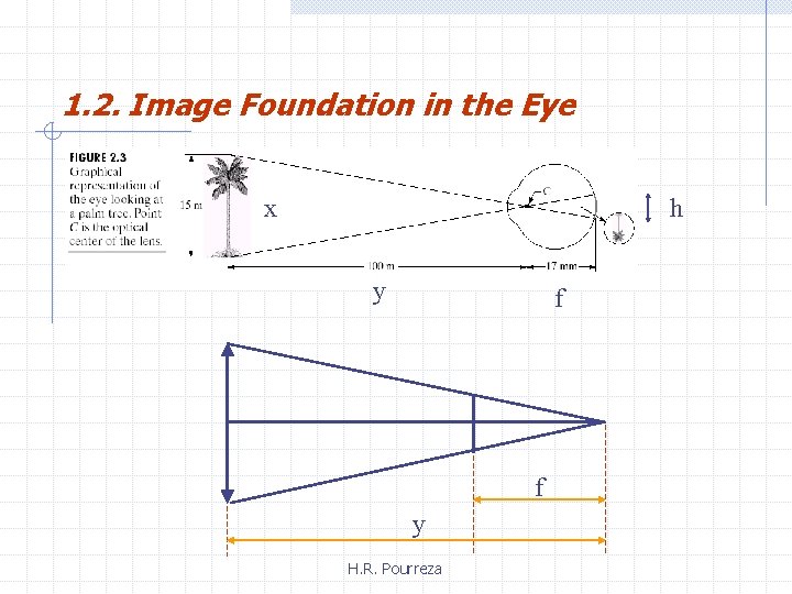
1. 2. Image Foundation in the Eye x h y f f y H. R. Pourreza

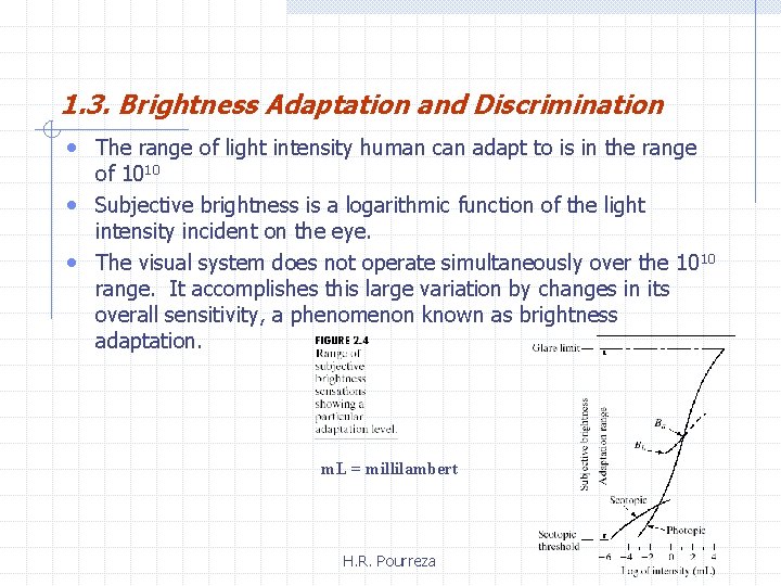
1. 3. Brightness Adaptation and Discrimination • The range of light intensity human can adapt to is in the range of 1010 • Subjective brightness is a logarithmic function of the light intensity incident on the eye. • The visual system does not operate simultaneously over the 1010 range. It accomplishes this large variation by changes in its overall sensitivity, a phenomenon known as brightness adaptation. m. L = millilambert H. R. Pourreza

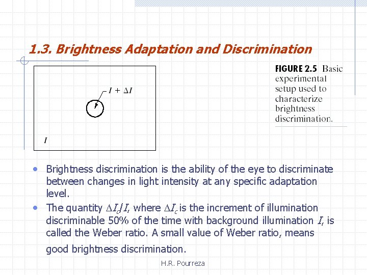
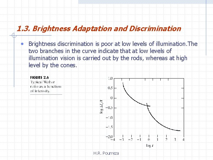
1. 3. Brightness Adaptation and Discrimination • Brightness discrimination is the ability of the eye to discriminate between changes in light intensity at any specific adaptation level. • The quantity Ic/I, where Ic is the increment of illumination discriminable 50% of the time with background illumination I, is called the Weber ratio. A small value of Weber ratio, means good brightness discrimination. H. R. Pourreza

1. 3. Brightness Adaptation and Discrimination • Brightness discrimination is poor at low levels of illumination. The two branches in the curve indicate that at low levels of illumination vision is carried out by the rods, whereas at high level by the cones. H. R. Pourreza

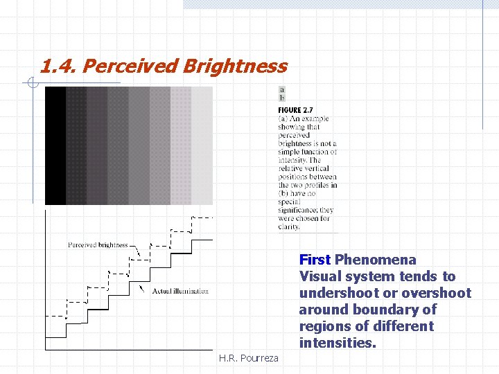
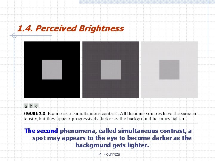
1. 4. Perceived Brightness Two phenomena clearly demonstrate that perceived brightness is not a simple function of intensity. H. R. Pourreza

1. 4. Perceived Brightness First Phenomena Visual system tends to undershoot or overshoot around boundary of regions of different intensities. H. R. Pourreza

1. 4. Perceived Brightness The second phenomena, called simultaneous contrast, a spot may appears to the eye to become darker as the background gets lighter. H. R. Pourreza

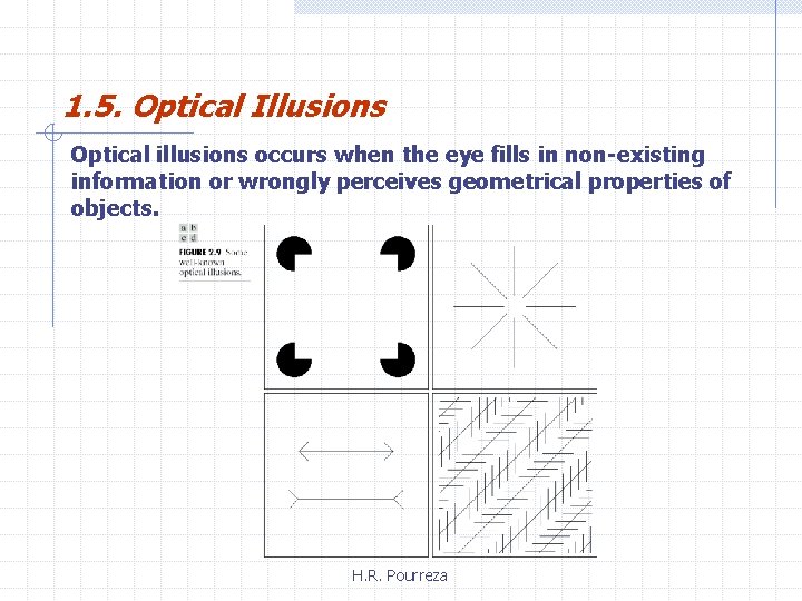
1. 5. Optical Illusions Optical illusions occurs when the eye fills in non-existing information or wrongly perceives geometrical properties of objects. H. R. Pourreza

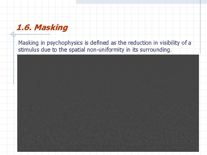
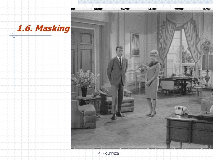
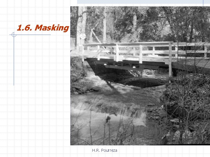
1. 6. Masking in psychophysics is defined as the reduction in visibility of a stimulus due to the spatial non-uniformity in its surrounding. H. R. Pourreza

1. 6. Masking H. R. Pourreza

1. 6. Masking H. R. Pourreza

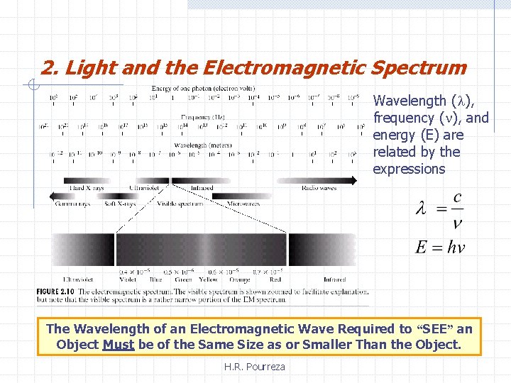
2. Light and the Electromagnetic Spectrum Wavelength ( ), frequency ( ), and energy (E) are related by the expressions The Wavelength of an Electromagnetic Wave Required to “SEE” an Object Must be of the Same Size as or Smaller Than the Object. H. R. Pourreza

2. Light and the Electromagnetic Spectrum • The colors that humans perceive in an object are determined by the nature of the light reflected from the object. • Achromatic or monochromatic light is void of color, and is described by its intensity (gray level). • Chromatic light spans the electromagnetic energy spectrum from 0. 43 to 0. 79 m, and is described by n Radiance: Total amount of energy that flows from the light source, and measured in watts (W) n Luminance: Measured in lumens (lm), gives a measure of the amount of energy an observer perceives from a light source n Brightness: Subjective descriptor of light perception that is practically impossible to measure. H. R. Pourreza

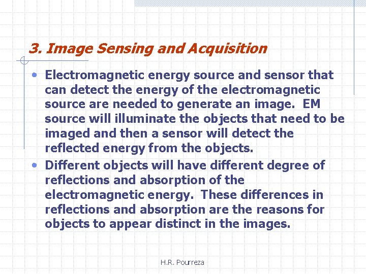
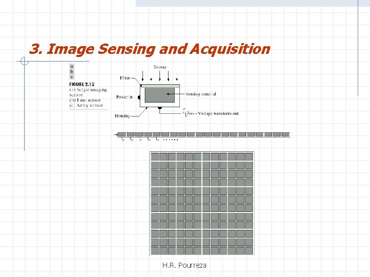
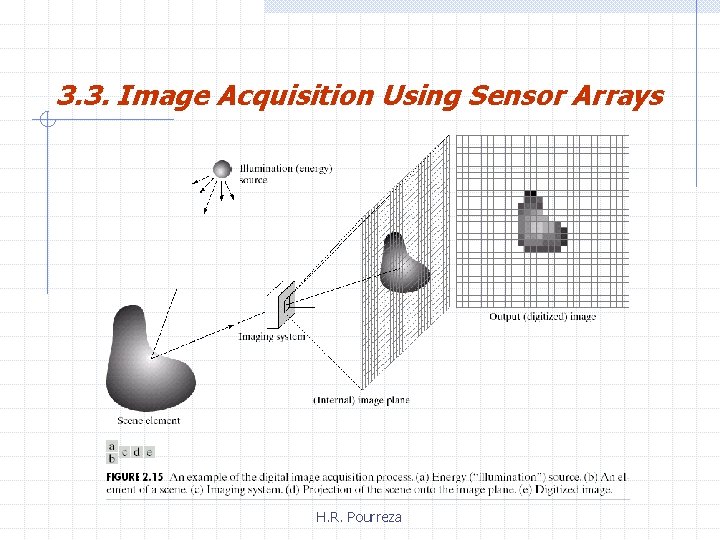
3. Image Sensing and Acquisition • Electromagnetic energy source and sensor that can detect the energy of the electromagnetic source are needed to generate an image. EM source will illuminate the objects that need to be imaged and then a sensor will detect the reflected energy from the objects. • Different objects will have different degree of reflections and absorption of the electromagnetic energy. These differences in reflections and absorption are the reasons for objects to appear distinct in the images. H. R. Pourreza

3. Image Sensing and Acquisition H. R. Pourreza

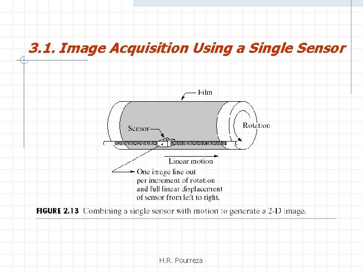
3. 1. Image Acquisition Using a Single Sensor H. R. Pourreza

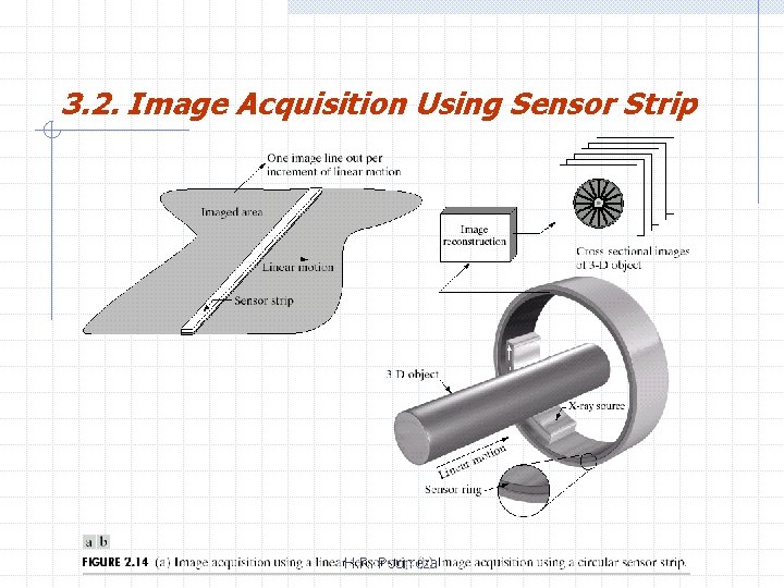
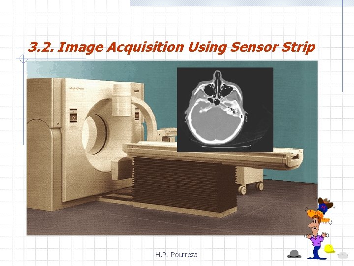
3. 2. Image Acquisition Using Sensor Strip H. R. Pourreza

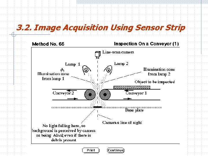
3. 2. Image Acquisition Using Sensor Strip • Measure the width of objects • Where we may be imaging and inspecting a continuous web of material flowing by the camera H. R. Pourreza

3. 2. Image Acquisition Using Sensor Strip H. R. Pourreza

3. 2. Image Acquisition Using Sensor Strip H. R. Pourreza

3. 3. Image Acquisition Using Sensor Arrays H. R. Pourreza

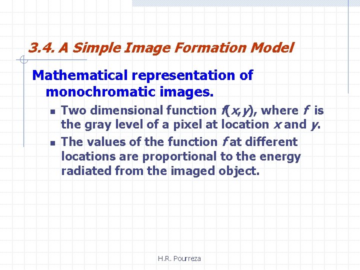
3. 4. A Simple Image Formation Model Mathematical representation of monochromatic images. n n Two dimensional function f(x, y), where f is the gray level of a pixel at location x and y. The values of the function f at different locations are proportional to the energy radiated from the imaged object. H. R. Pourreza

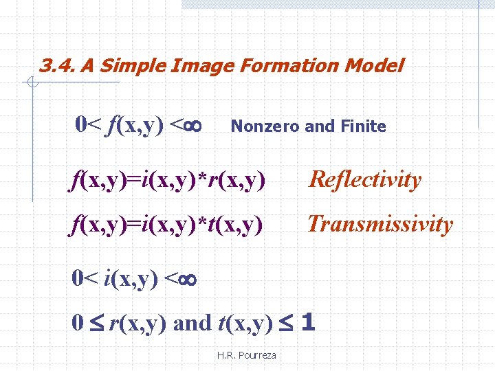
3. 4. A Simple Image Formation Model 0< f(x, y) < Nonzero and Finite f(x, y)=i(x, y)*r(x, y) Reflectivity f(x, y)=i(x, y)*t(x, y) Transmissivity 0< i(x, y) < 0 r(x, y) and t(x, y) 1 H. R. Pourreza

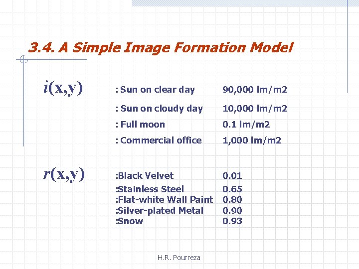
3. 4. A Simple Image Formation Model i(x, y) r(x, y) : Sun on clear day 90, 000 lm/m 2 : Sun on cloudy day 10, 000 lm/m 2 : Full moon 0. 1 lm/m 2 : Commercial office 1, 000 lm/m 2 : Black Velvet : Stainless Steel : Flat-white Wall Paint : Silver-plated Metal : Snow 0. 01 0. 65 0. 80 0. 93 H. R. Pourreza

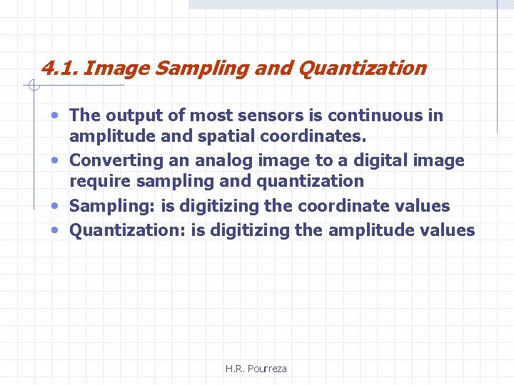
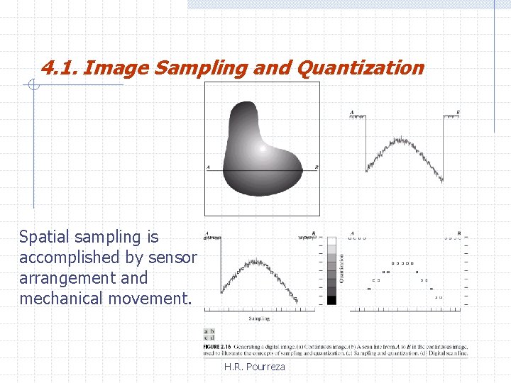
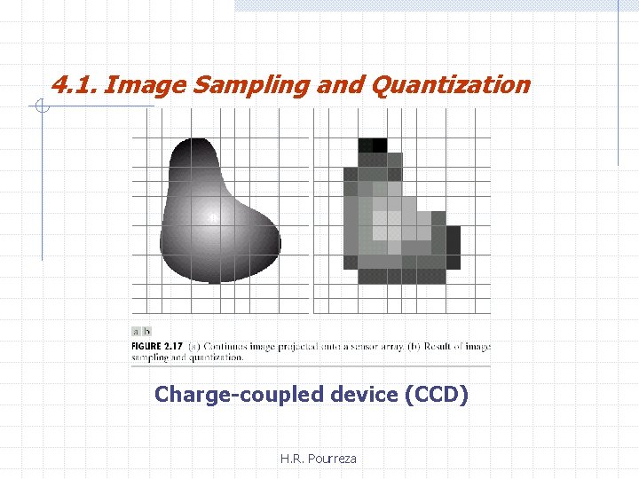
4. 1. Image Sampling and Quantization • The output of most sensors is continuous in amplitude and spatial coordinates. • Converting an analog image to a digital image require sampling and quantization • Sampling: is digitizing the coordinate values • Quantization: is digitizing the amplitude values H. R. Pourreza

4. 1. Image Sampling and Quantization Spatial sampling is accomplished by sensor arrangement and mechanical movement. H. R. Pourreza

4. 1. Image Sampling and Quantization Charge-coupled device (CCD) H. R. Pourreza

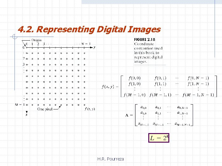
4. 2. Representing Digital Images H. R. Pourreza

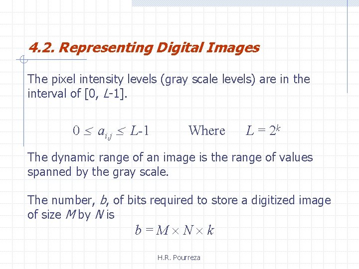
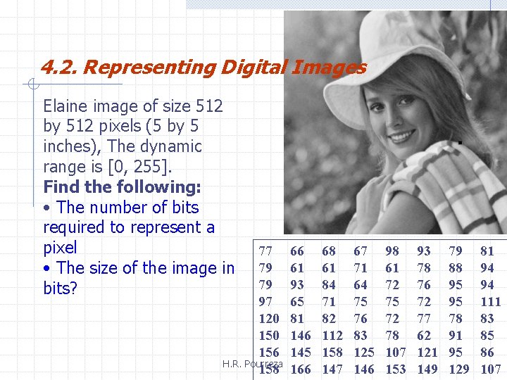
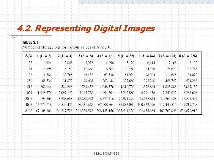
4. 2. Representing Digital Images The pixel intensity levels (gray scale levels) are in the interval of [0, L-1]. 0 ai, j L-1 Where L = 2 k The dynamic range of an image is the range of values spanned by the gray scale. The number, b, of bits required to store a digitized image of size M by N is b=M N k H. R. Pourreza

4. 2. Representing Digital Images Elaine image of size 512 by 512 pixels (5 by 5 inches), The dynamic range is [0, 255]. Find the following: • The number of bits required to represent a pixel • The size of the image in bits? 77 79 79 97 120 156 H. R. Pourreza 158 66 61 93 65 81 146 145 166 68 61 84 71 82 112 158 147 67 71 64 75 76 83 125 146 98 61 72 75 72 78 107 153 93 78 76 72 77 62 121 149 79 88 95 95 78 91 95 129 81 94 94 111 83 85 86 107

4. 2. Representing Digital Images H. R. Pourreza

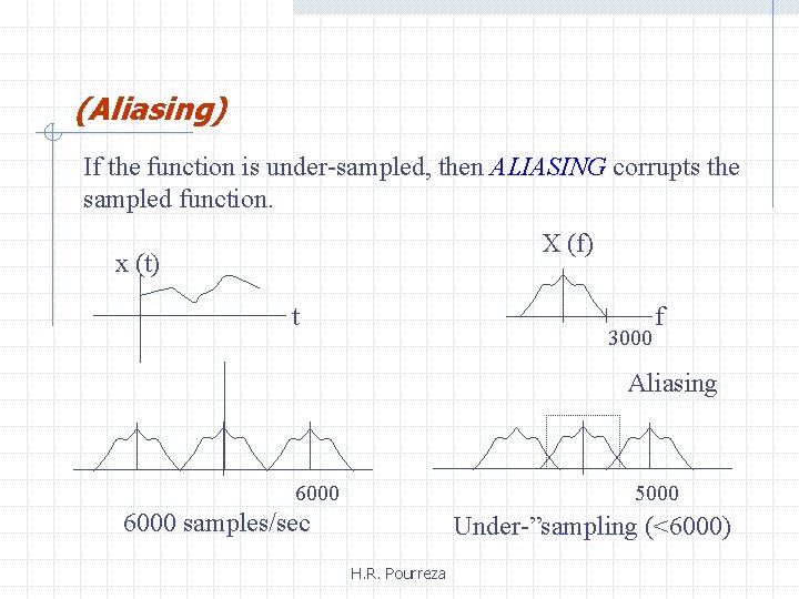
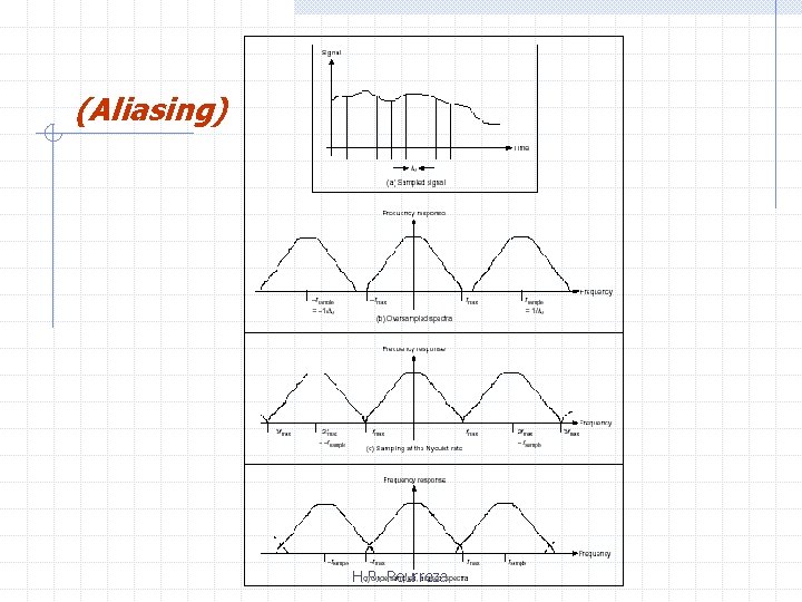
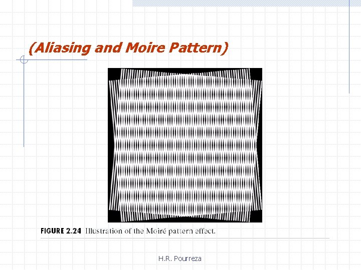
(Sampling Theorem and Aliasing Effect) Shannon sampling theorem states that if a function is sampled at a rate equal to or greater than twice its highest frequency, it is possible to recover completely the original function from its samples. H. R. Pourreza

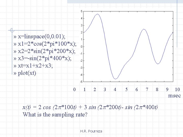
» x=linspace(0, 0. 01); » x 1=2*cos(2*pi*100*x); » x 2=2*sin(2*pi*200*x); » x 3=-sin(2*pi*400*x); » xt=x 1+x 2+x 3; » plot(xt) 0 1 2 3 4 5 6 7 8 x(t) = 2 cos (2 *100 t) + 3 sin (2 *200 t)- sin (2 *400 t) What is the sampling rate? H. R. Pourreza 9 10 msec

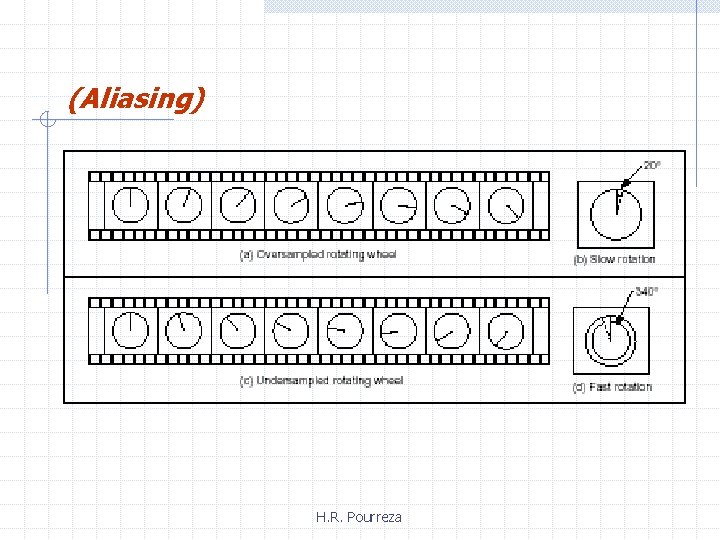
(Aliasing) If the function is under-sampled, then ALIASING corrupts the sampled function. X (f) x (t) t 3000 f Aliasing 6000 5000 6000 samples/sec Under-”sampling (<6000) H. R. Pourreza

(Aliasing) H. R. Pourreza

(Aliasing) H. R. Pourreza

(Aliasing) H. R. Pourreza

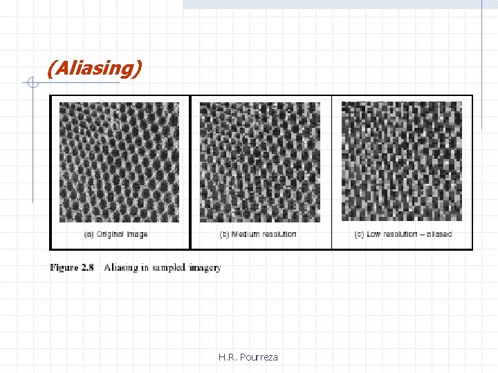
(Aliasing and Moire Pattern) H. R. Pourreza

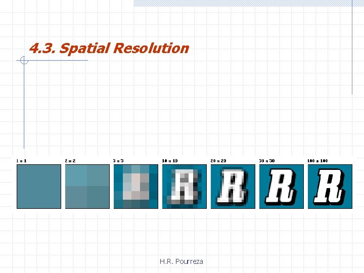
4. 3. Spatial Resolution H. R. Pourreza

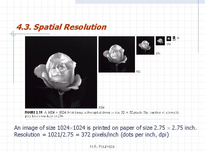
4. 3. Spatial Resolution An image of size 1024 is printed on paper of size 2. 75 inch. Resolution = 1021/2. 75 = 372 pixels/inch (dots per inch, dpi) H. R. Pourreza

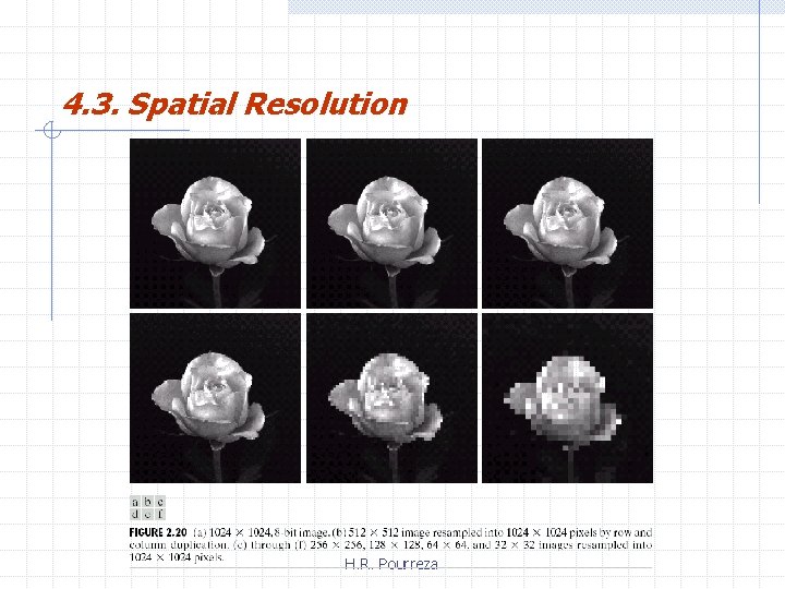
4. 3. Spatial Resolution H. R. Pourreza

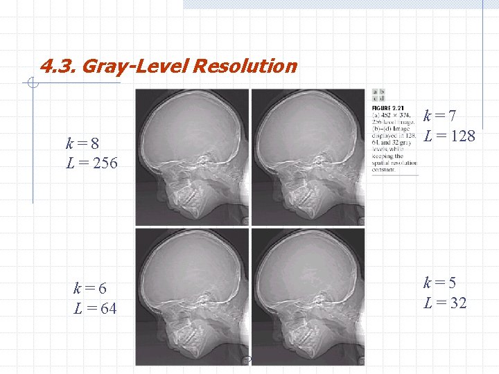
4. 3. Gray-Level Resolution k=7 L = 128 k=8 L = 256 k=5 L = 32 k=6 L = 64 H. R. Pourreza

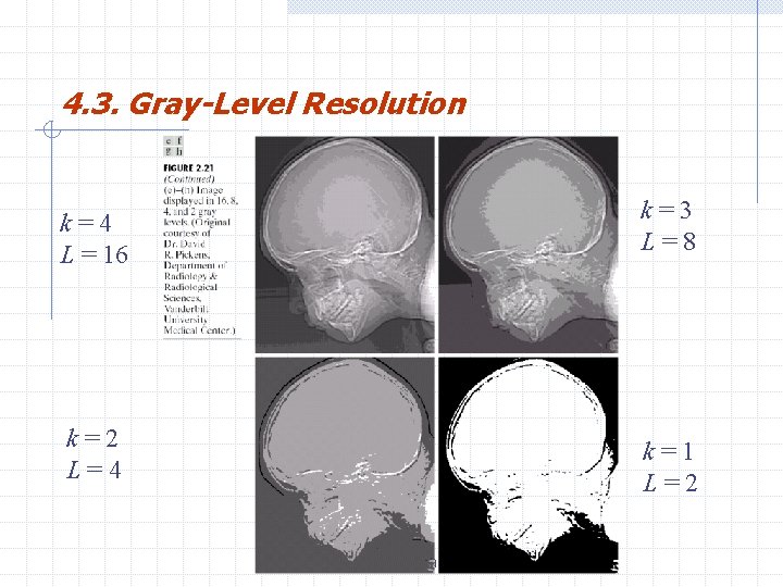
4. 3. Gray-Level Resolution k=4 L = 16 k=3 L=8 k=2 L=4 k=1 L=2 H. R. Pourreza

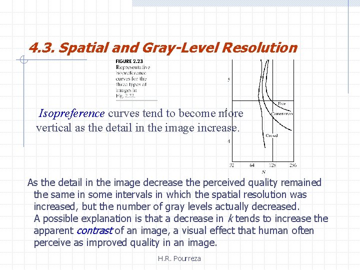
4. 3. Spatial and Gray-Level Resolution Huang Experiment [1965] attempt to quantify experimentally the effects on image quality produced by varying N and k simultaneously. H. R. Pourreza

4. 3. Spatial and Gray-Level Resolution Isopreference curves tend to become more vertical as the detail in the image increase. As the detail in the image decrease the perceived quality remained the same in some intervals in which the spatial resolution was increased, but the number of gray levels actually decreased. A possible explanation is that a decrease in k tends to increase the apparent contrast of an image, a visual effect that human often perceive as improved quality in an image. H. R. Pourreza

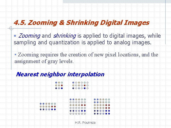
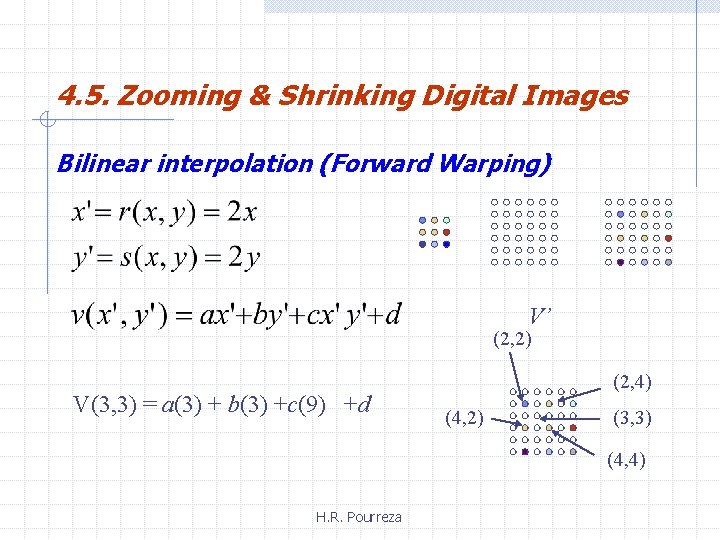
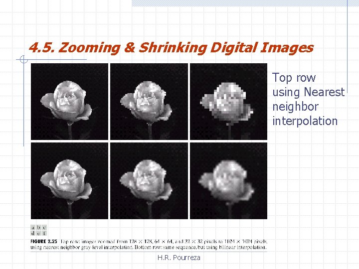
4. 5. Zooming & Shrinking Digital Images • Zooming and shrinking is applied to digital images, while sampling and quantization is applied to analog images. • Zooming requires the creation of new pixel locations, and the assignment of gray levels. Nearest neighbor interpolation H. R. Pourreza

4. 5. Zooming & Shrinking Digital Images Bilinear interpolation (Forward Warping) V’ (2, 2) V(3, 3) = a(3) + b(3) +c(9) +d (2, 4) (4, 2) (3, 3) (4, 4) H. R. Pourreza

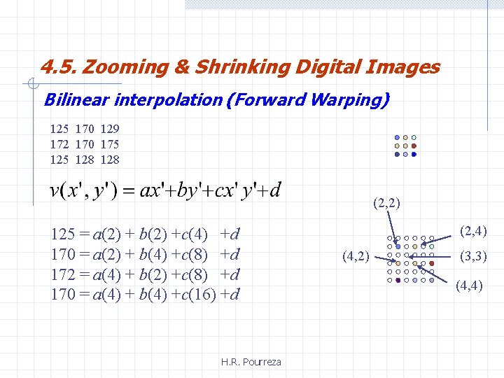
4. 5. Zooming & Shrinking Digital Images Bilinear interpolation (Forward Warping) 125 170 129 172 170 175 128 128 (2, 2) 125 = a(2) + b(2) +c(4) +d 170 = a(2) + b(4) +c(8) +d 172 = a(4) + b(2) +c(8) +d 170 = a(4) + b(4) +c(16) +d H. R. Pourreza (2, 4) (4, 2) (3, 3) (4, 4)

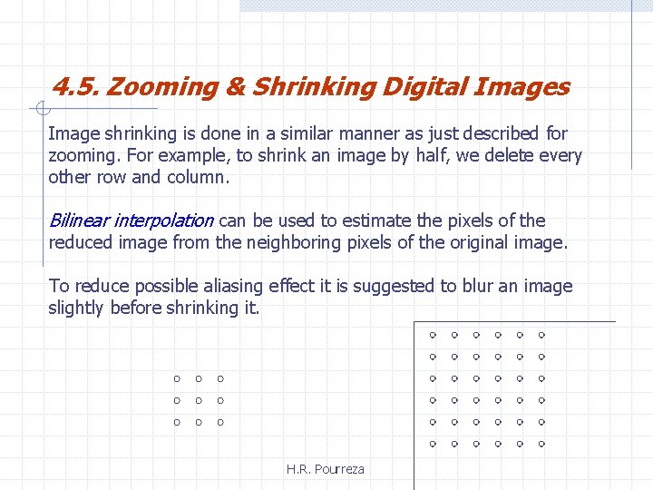
4. 5. Zooming & Shrinking Digital Images Image shrinking is done in a similar manner as just described for zooming. For example, to shrink an image by half, we delete every other row and column. Bilinear interpolation can be used to estimate the pixels of the reduced image from the neighboring pixels of the original image. To reduce possible aliasing effect it is suggested to blur an image slightly before shrinking it. H. R. Pourreza

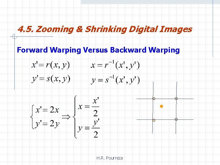
4. 5. Zooming & Shrinking Digital Images Forward Warping Versus Backward Warping H. R. Pourreza

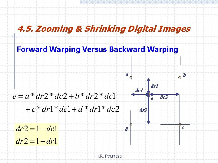
4. 5. Zooming & Shrinking Digital Images Forward Warping Versus Backward Warping a b dc 1 dr 1 e dc 2 dr 2 d H. R. Pourreza c

4. 5. Zooming & Shrinking Digital Images Top row using Nearest neighbor interpolation H. R. Pourreza

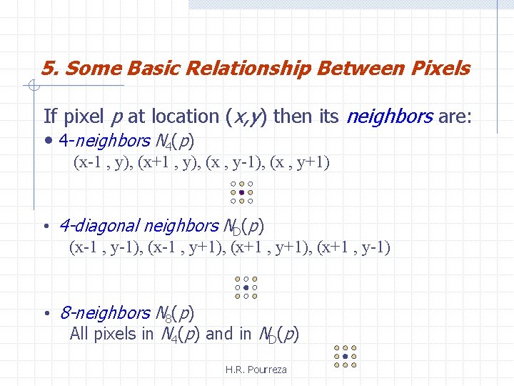
5. Some Basic Relationship Between Pixels If pixel p at location (x, y) then its neighbors are: • 4 -neighbors N 4(p) (x-1 , y), (x+1 , y), (x , y-1), (x , y+1) • 4 -diagonal neighbors ND(p) (x-1 , y-1), (x-1 , y+1), (x+1 , y-1) • 8 -neighbors N 8(p) All pixels in N 4(p) and in ND(p) H. R. Pourreza

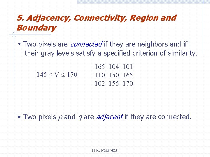
5. Adjacency, Connectivity, Region and Boundary • Two pixels are connected if they are neighbors and if their gray levels satisfy a specified criterion of similarity. 145 < V 170 165 104 101 110 150 165 102 155 170 • Two pixels p and q are adjacent if they are connected. H. R. Pourreza

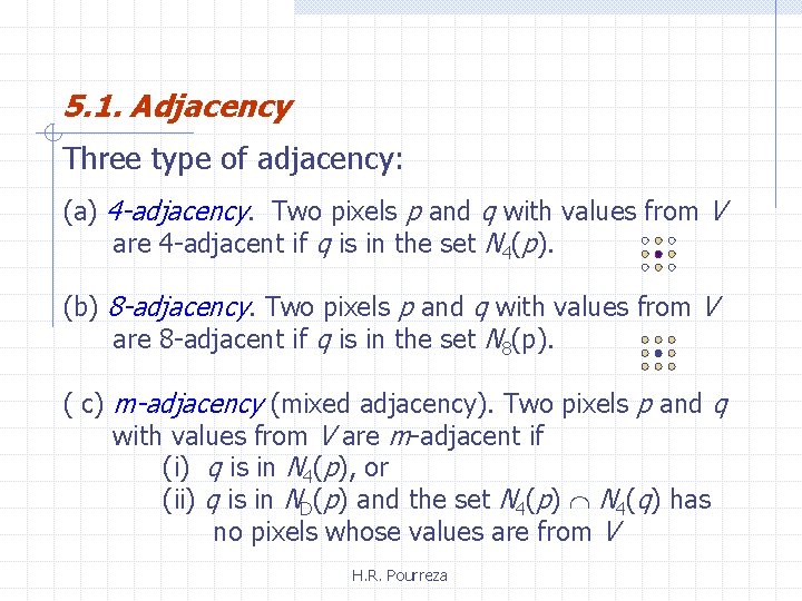
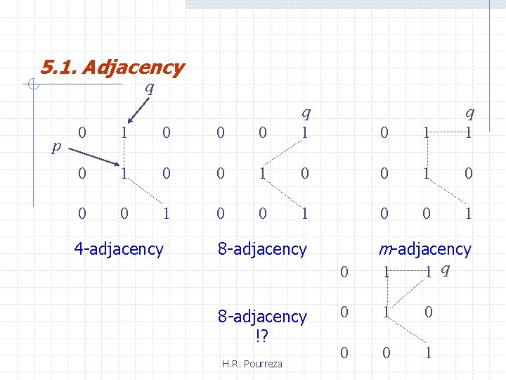
5. 1. Adjacency Three type of adjacency: (a) 4 -adjacency. Two pixels p and q with values from V are 4 -adjacent if q is in the set N 4(p). (b) 8 -adjacency. Two pixels p and q with values from V are 8 -adjacent if q is in the set N 8(p). ( c) m-adjacency (mixed adjacency). Two pixels p and q with values from V are m-adjacent if (i) q is in N 4(p), or (ii) q is in ND(p) and the set N 4(p) N 4(q) has no pixels whose values are from V H. R. Pourreza

5. 1. Adjacency q p 0 1 0 0 0 q 1 0 0 1 0 0 1 4 -adjacency H. R. Pourreza 1 m-adjacency 8 -adjacency !? 0 q 1 0 1 1 q 0 1 0 0 0 1

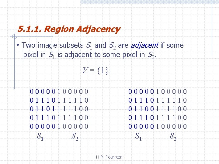
5. 1. 1. Region Adjacency • Two image subsets S 1 and S 2 are adjacent if some pixel in S 1 is adjacent to some pixel in S 2. V = {1} 00000100000 0111110 01101111100 0111100 00000100000 S 1 00000100000 0111110 01100111100 00000100000 S 2 S 1 H. R. Pourreza S 2

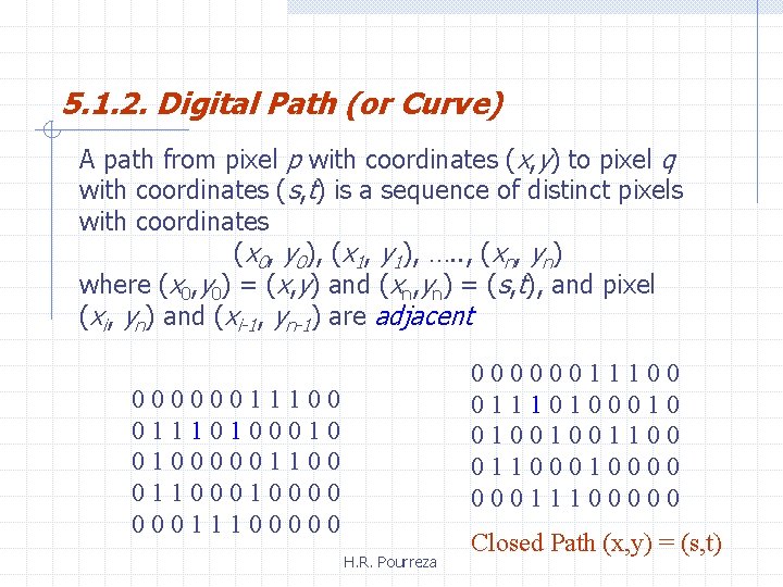
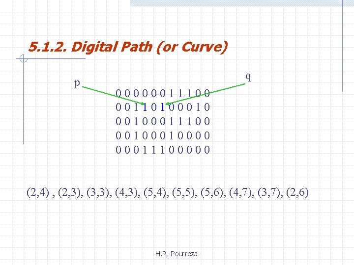
5. 1. 2. Digital Path (or Curve) A path from pixel p with coordinates (x, y) to pixel q with coordinates (s, t) is a sequence of distinct pixels with coordinates (x 0, y 0), (x 1, y 1), …. . , (xn, yn) where (x 0, y 0) = (x, y) and (xn, yn) = (s, t), and pixel (xi, yn) and (xi-1, yn-1) are adjacent 00000011100 01110100010 0100100110000 00011100000011100 01110100010 0100000110000 00011100000 H. R. Pourreza Closed Path (x, y) = (s, t)

5. 1. 2. Digital Path (or Curve) p q 00000011100 001101000100011100 0010000 00011100000 (2, 4) , (2, 3), (3, 3), (4, 3), (5, 4), (5, 5), (5, 6), (4, 7), (3, 7), (2, 6) H. R. Pourreza

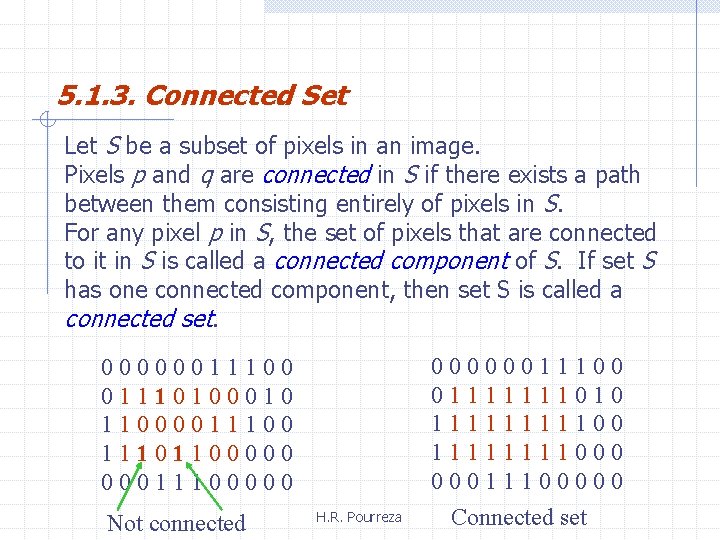
5. 1. 3. Connected Set Let S be a subset of pixels in an image. Pixels p and q are connected in S if there exists a path between them consisting entirely of pixels in S. For any pixel p in S, the set of pixels that are connected to it in S is called a connected component of S. If set S has one connected component, then set S is called a connected set. 00000011100 01110100010 11000011100 11101100000 00011100000 Not connected H. R. Pourreza 00000011100 01111111010 11111000 00011100000 Connected set

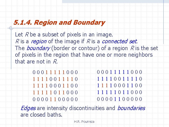
5. 1. 4. Region and Boundary Let R be a subset of pixels in an image. R is a region of the image if R is a connected set. The boundary (border or contour) of a region R is the set of pixels in the region that have one or more neighbors that are not in R. 00011111000 11110011110001100 11111011000 00001100000 Edges are intensity discontinuities and boundaries are closed baths. H. R. Pourreza

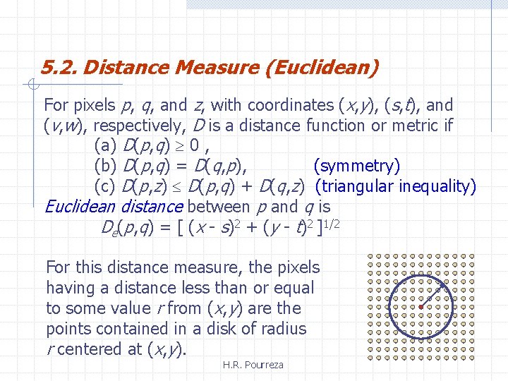
5. 2. Distance Measure (Euclidean) For pixels p, q, and z, with coordinates (x, y), (s, t), and (v, w), respectively, D is a distance function or metric if (a) D(p, q) 0 , (b) D(p, q) = D(q, p), (symmetry) (c) D(p, z) D(p, q) + D(q, z) (triangular inequality) Euclidean distance between p and q is De(p, q) = [ (x - s)2 + (y - t)2 ]1/2 For this distance measure, the pixels having a distance less than or equal to some value r from (x, y) are the points contained in a disk of radius r centered at (x, y). H. R. Pourreza

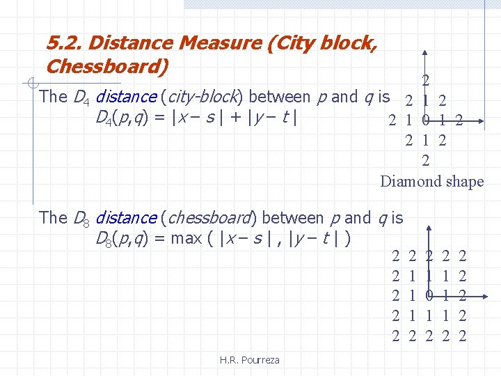
5. 2. Distance Measure (City block, Chessboard) 2 The D 4 distance (city-block) between p and q is 2 1 2 D 4 ( p , q ) = | x – s | + | y – t | 2 1 0 1 2 2 Diamond shape The D 8 distance (chessboard) between p and q is D 8(p, q) = max ( |x – s | , |y – t | ) 2 2 2 H. R. Pourreza 2 1 1 1 2 2 1 0 1 2 2 1 1 1 2 2 2

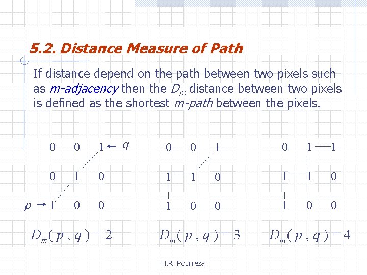
5. 2. Distance Measure of Path If distance depend on the path between two pixels such as m-adjacency then the Dm distance between two pixels is defined as the shortest m-path between the pixels. p 0 0 1 1 0 q 0 0 1 1 0 0 1 0 0 D m( p , q ) = 2 D m( p , q ) = 3 H. R. Pourreza D m( p , q ) = 4

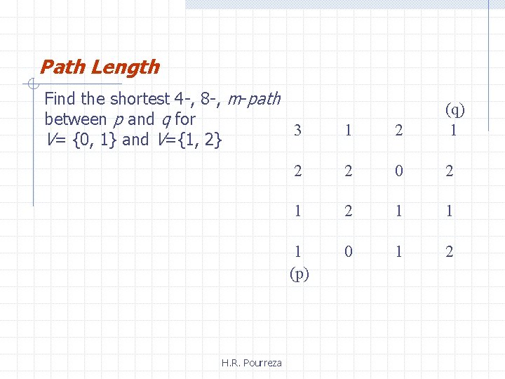
Path Length Find the shortest 4 -, 8 -, m-path between p and q for 3 V= {0, 1} and V={1, 2} H. R. Pourreza 1 2 (q) 1 2 2 0 2 1 1 1 (p) 0 1 2

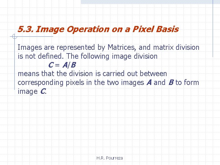
5. 3. Image Operation on a Pixel Basis Images are represented by Matrices, and matrix division is not defined. The following image division C = A /B means that the division is carried out between corresponding pixels in the two images A and B to form image C. H. R. Pourreza

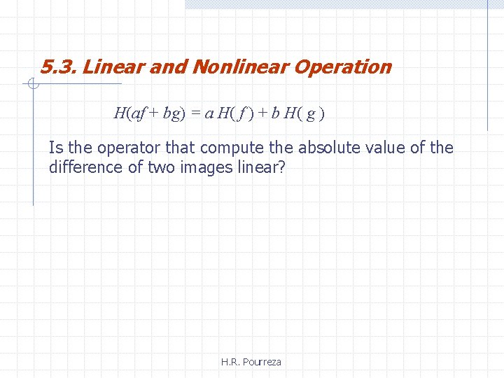
5. 3. Linear and Nonlinear Operation H(af + bg) = a H( f ) + b H( g ) Is the operator that compute the absolute value of the difference of two images linear? H. R. Pourreza