Laboratorio Metodi di Potenziale Prof Carla Braitenberg Laboratorio

Laboratorio Metodi di Potenziale Prof. Carla Braitenberg Laboratorio Dott. Tommaso Pivetta, Dott. Alberto Pastorutti AA. 2020 -2021 Università di Trieste

Utilizzare per articoli: scopus, google scholar. • • • • Articolo: Gmt Tattoni (da definire) Mino ary (da definire) Caravati (da definire) Galleonardo matteo Bacino Pannonico Vattovaz michelle Mare di Ross Antartide Markezic Nora Africa Nord-occidentale. Western African Craton Luppino Dario Costa Cile. Beltrame Chantal Norvegia Fenu Federica Isole Britanniche Chinelatto Letizia Tibet. Zukon Elen Islanda Taverna Perla Giappone Giordano Fabio Cratere di Yukatan, Chicxulub crater

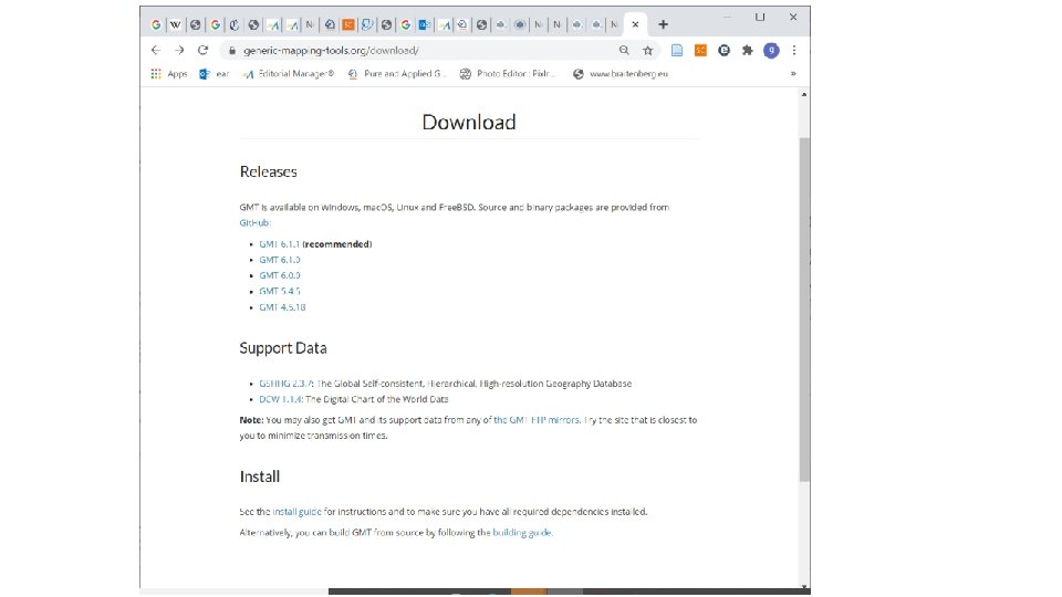
Install GMT 6. 1. 1 • You must install GMT on your PC for the laboratory. At the course windows system is used. If your system is different from Windows, please use the PCs of the University or install a Windows partition on your pc. • GMT is a versatile tool for mapping and modeling the potential field data. We will use it to display the gravity and magnetic fields. • Download link: https: //www. generic-mapping-tools. org/download/ • The mapping tool is a collection of single routines which are called from the command line. They read input data and create an output plot file (default is postscript). To display the plot file you must launch a secondary program that reads the postscript file. • gmt-6. 1. 1 -darwin-x 86_64. dmg (installer for Mac) • gmt-6. 1. 1 -win 64 (installer for Windows) • gmt-6. 1. 1 -win 32 (installer for Windows)

GMT other useful links • Link al software: http: //gmt. soest. hawaii. edu/projects/gmt/wiki/Installing • Link alla documentazione: • https: //docs. generic-mapping-tools. org/6. 1/ • E’ consigliato installare un programma per la lettura dei file in formato Postscript: gv (ftp: //ftp. gnu. org/gnu/gv/) o ghostview • Anche un buon editor di testo, come Notepad++ • https: //qpdownload. com/notepad-plus/

The files offered for download

Double click on the win 32 or win 64. exe file

By default the GMT 6. 1 is installed under the directory programs. In my example I also have the previous version GMT 5 installed.

You need a postscript viewer. GMT recommends Post. Script previewer (e. g. , gv (or ghostview or plain ghostscript)) Once the ghostview has installed (for instance in C: Programmi), please copy the folder gs to the folder c: programs

Install ghostscript into the prgrams folder. When he asks where to install, indicate: c: programs

The documentation and examples of GMT are stored in the folder doc • C: programsgmt 6sharedoc • The subfolder html contains a tutorial and the full instructions on how to use the routines • Double-click on GMT_Tutorial. html for a tutorial or GMT_Docs for a full documentation.

To run the GMT routines open a command line window. You can type cmd. The GMT routines are must be actively run by a script. The script contains the series of routines that must be launched one after the other. You will not have the possibility to launch the programs on a windows based interface. This has some advantages: if you must do the similar graph many times, then it is an advantage tpo have coded the steps in a script.

By typing the command gmt on the command line the below text is diplayed. It means that GMT was installed correctly on your pc.

It is necessary that your PC has the correct international settings of how to display numbers

You must set the decimal separator to dot, not comma. Here the default settings, which are not ok for GMT.

After you have corrected the settings you should have the following:

For launching the GMT commands, save the commands to a script you have edited in notepad++. Save all scripts in the folder C: MEPO. Please create a working folder C: MEPOinput_data. To be executable the script must end with the extension myscript. bat. Double click on the bat-file will launch the script. The following script will create the map you see in the next slide. Install the program Notepad++ for editing the scripts. • gmt pscoast -R-90/-70/0/20 -JM 6 i -P -Ba -Gchocolate > GMT_tut_3. ps • C: programsgs 9. 53. 3bingswin 64 GMT_tut_3. ps

From the GMT tutorial • gmt pscoast -R-90/-70/0/20 -JM 6 i -P -Ba -Gchocolate > GMT_tut_3. ps • C: programsgs 9. 53. 3bingswin 64 GMT_tut_3. ps

Explanation of the pscoast command. • pscoast -R-5/10/-5/5 -JM 6 i -P -Ba -Gchocolate > Mepo_Es 1. ps • -R-5/10/-5/5: estremi in longitudine e tatitudine • -JM 6 i: proezione di mercatore. Mappa larga 6 inch • -P: portrait (orientazione della carta) • -Ba: annotazione degli assi • -Gchocolate: terre emerse in beige • > Mepo_Es 1. ps: output su file di tipo post-script

Mappa di Coste con coordinate • psbasemap -R-5/10/-5/5 -JM 6 i -P -Ba -B+t"Esercizio 2" -K > Mepo_Es 2. ps • Psbasemap: mappa di base con le coordinate • > apri file di uscita • >> continua a scrivere sullo stesso file • -K: arrivera’ altro materiale per il file • pscoast -R-5/10/-5/5 -JM 6 i -P –Ba -Gchocolate -O >> Mepo_Es 2. ps • -O: overlay sul file precedente

Ulteriori approfondimenti: • Leggere la documentazione delle singole istruzioni sul sito GMT • Creare ulteriori mappe • Creare mappa globale delle coste, utilizzando altre proiezioni geografiche. Si veda il GMT tutorial 1: • http: //gmt. soest. hawaii. edu/doc/5. 3. 2/GMT_Tutorial. html#sessionone

Indice degli argomenti da trattare durante il laboratorio 1 Installazione e primo utilizzo del pacchetto software GMT (General Mapping Tools). Installare anche database di topografia e coste e fiumi. Creazione di mappe con topografia e coste. 2 Creazione di mappe di: anomalia di gravita’ , Bouguer e topografia per zona a scelta dello studente. Recupero dati dal database ICGEM

Recuperare i dati dal sito ICGEM • Le schede successive illustrano come creare i dati di gravita’ dal sito ICGEM e rappresentarli graficamente in GMT. • http: //icgem. gfz-potsdam. de/home

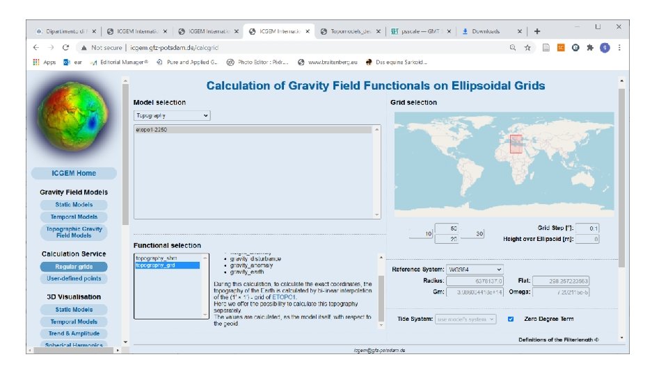
Calculate the gravity anomaly at zero height for a static gravity field model in spherical harmonics. Use model XGM 2019 e_2159, choose classic gravity anomaly. For definition of the functionals the user guide of the ICGEM page.

You must download the grid. You will find the grid in the download folder. Please copy it to your working folder c: MEPOdati_input. The next slide shows the header of the file. You can open the file in Notepad++.

The header contains all the information abut the spherical harmonic model used to make the calculations, the parameters used. Check the number of lines use by the header- the number of lines must be known when we intend to read the file in GMT.

Convert column format to grid format of GMT and plot • xyz 2 grd. input_data grav_Anom_cl. gdf G. input_dataGrav. Anom_Cl. grd -h 35 -I 0. 1/0. 1 R 10/30/20/50 -V • grdinfo. input_dataGrav. Anom_Cl. grd latlimit_north latlimit_south longlimit_west longlimit_east 50. 000000 20. 000000 10. 000000 30. 000000 End 13. 01. 2021

Plot the grid as contour lines and color plot. Here the coastline is drawn. • xyz 2 grd. input_datagrav_Anom_cl. gdf -G. input_dataGrav. Anom_Cl. grd -h 35 -I 0. 1/0. 1 -R 10/30/20/50 -V • grdinfo. input_dataGrav. Anom_Cl. grd • psbasemap -R 10/30/20/50 -JM 5 i -P -Ba -B+t"Gravity Anomaly" -K > Mepo_Es 1 b. ps • • grd 2 cpt. input_dataGrav. Anom_Cl. grd -Crainbow -L-180/180 -Z > tess. cpt grdimage -R 10/30/20/50. input_dataGrav. Anom_Cl. grd -Ctess. cpt -JM 5 i -O -K >> Mepo_Es 1 b. ps pscoast -R 10/30/20/50 -JM 5 i -I 1 -Na -W 0. 8 p -Dh -P -Ba -O -K >> Mepo_Es 1 b. ps grdcontour. input_dataGrav. Anom_Cl. grd -R 10/30/20/50 -JM 5 i -C 30 -O >> Mepo_Es 1 b. ps • C: programsgs 9. 53. 3bingswin 64 -s. DEVICE=jpeg -d. Use. Crop. Box -r 300 -s. Output. File=Mepo_Es 1 b. jpg Mepo_Es 1 b. ps

Plot the grid as contour lines on top of the basemap and save as figure in. jpg format • psbasemap -R 10/30/20/50 -JM 5 i -P -Ba -B+t"Gravity Anomaly" -K > Mepo_Es 1. ps • grd 2 cpt. input_dataGrav. Anom_Cl. grd -Crainbow -L-180/180 -Z > tess. cpt • pscoast -R 10/30/20/50 -JM 5 i -I 1 -Na -Ggray -Dh -P -Ba -O -K >> Mepo_Es 1. ps • grdcontour. input_dataGrav. Anom_Cl. grd -R 10/30/20/50 -JM 5 i -C 30 -O >> Mepo_Es 1. ps • C: programsgs 9. 53. 3bingswin 64 -s. DEVICE=jpeg -d. Use. Crop. Box -r 300 s. Output. File=Mepo_Es 1. jpg Mepo_Es 1. ps

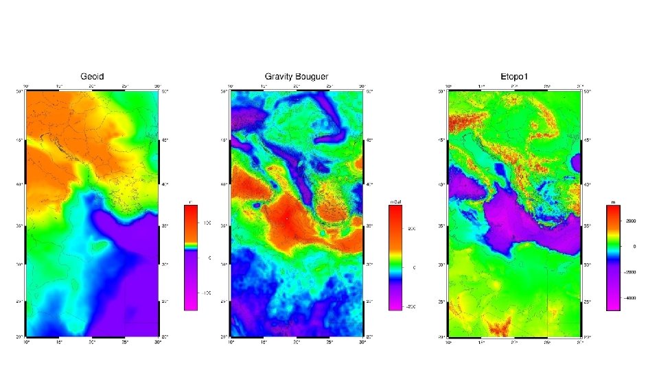
Resulting maps of previous scripts

The ICGEM calculation service allows to calculate also other functionals. Calculate the Bouguer field (simple Bouguer), the geoid, and the topography for the same area. Leave limits and gravity model the same. Here the screen for the simple Bouguer anomaly.

Download grid and rename it as for instance: XGM 2019_grav. BG. gdf. You will find the file in your downloads folder. Copy the file to your working directory. This name must be consistent with the name in the next script

Plot the Bouguer as contour lines on top of the basemap. • xyz 2 grd. input_dataXGM 2019_grav. BG. gdf -G. input_dataGrav. Anom_BG. grd -h 37 -I 0. 1/0. 1 -R 10/30/20/50 -V • grdinfo. input_dataGrav. Anom_BG. grd • psbasemap -R 10/30/20/50 -JM 5 i -P -Ba -B+t"Gravity Bouguer" -K > Mepo_Es 1_BG. ps • • • grd 2 cpt. input_dataGrav. Anom_BG. grd -Crainbow -L-220/320 -Z > tess. cpt grdimage -R 10/30/20/50. input_dataGrav. Anom_BG. grd -Ctess. cpt -JM 5 i -O -K >> Mepo_Es 1_BG. ps pscoast -R 10/30/20/50 -JM 5 i -I 1 -Na -W -Dh -P -Ba -O -K >> Mepo_Es 1_BG. ps grdcontour. input_dataGrav. Anom_Cl. grd -R 10/30/20/50 -JM 5 i -C 30 -O -K >> Mepo_Es 1_BG. ps psscale -Dx 6 i/1 i+w 4 i/0. 5 i -Ba -By 50+lm. Gal -Ctess. cpt -O >> Mepo_Es 1_BG. ps C: programsgs 9. 53. 3bingswin 64 -s. DEVICE=jpeg -d. Use. Crop. Box -r 300 -s. Output. File=Mepo_Es 1_BG. jpg Mepo_Es 1_BG. ps Attention, number of header lines is different!

create and plot the Geoid map • • • : : ------Geoid xyz 2 grd. input_dataXGM 2019_Geoid. gdf -G. input_dataGeoid. grd -h 36 -I 0. 1/0. 1 -R 10/30/20/50 -V grdinfo. input_dataGeoid. grd psbasemap -R 10/30/20/50 -JM 5 i -P -Ba -B+t"Geoid" -K > Mepo_Es 1_GE. ps grd 2 cpt. input_dataGeoid. grd -Crainbow -L-150/150 -Z > tess. cpt grdimage -R 10/30/20/50. input_dataGeoid. grd -Ctess. cpt -JM 5 i -O -K >> Mepo_Es 1_GE. ps pscoast -R 10/30/20/50 -JM 5 i -I 1 -Na -W -Dh -P -Ba -O -K >> Mepo_Es 1_GE. ps grdcontour. input_dataGeoid. grd -R 10/30/20/50 -JM 5 i -C 30 -O -K >> Mepo_Es 1_GE. ps psscale -Dx 6 i/1 i+w 4 i/0. 5 i -Ba -By 50+lm -Ctess. cpt -O >> Mepo_Es 1_GE. ps C: programsgs 9. 53. 3bingswin 64 -s. DEVICE=jpeg -d. Use. Crop. Box -r 300 s. Output. File=Mepo_Es 1_GE. jpg Mepo_Es 1_GE. ps

Create topography in ICGEM and plot it • • • : : ------Etopo 1 xyz 2 grd. input_dataetopo 1. gdf -G. input_dataEtopo 1_select. grd –h 29 -I 0. 1/0. 1 -R 10/30/20/50 -V grdinfo. input_dataEtopo 1_select. grd psbasemap -R 10/30/20/50 -JM 5 i -P -Ba -B+t"Etopo 1" -K > Mepo_Es 1_Topo. ps grd 2 cpt. input_dataEtopo 1_select. grd -Crainbow -L-5000/3200 -Z > tess. cpt grdimage -R 10/30/20/50. input_dataEtopo 1_select. grd -Ctess. cpt -JM 5 i -O -K >> Mepo_Es 1_Topo. ps pscoast -R 10/30/20/50 -JM 5 i -I 1 -Na -W -Dh -P -Ba -O -K >> Mepo_Es 1_Topo. ps grdcontour. input_dataEtopo 1_select. grd -R 10/30/20/50 -JM 5 i -C 500 -O >> Mepo_Es 1_Topo. ps psscale -Dx 6 i/1 i+w 4 i/0. 5 i -Ba -By 50+lm -Ctess. cpt -O >> Mepo_Es 1_Topo. ps C: programsgs 9. 53. 3bingswin 64 -s. DEVICE=jpeg -d. Use. Crop. Box -r 300 s. Output. File=Mepo_Es 1_Topo. jpg Mepo_Es 1_Topo. ps

Carta delle anomalie di Bouguer • Dominata in termini di ampiezza da anomalie sotto le Alpi • Sotto le Alpi c’è una mancanza di massa • Vogliamo verificare se è ‘giustificabile’ dall’effetto isostatico

Isostasia secondo Airy Bilancio isostatico a terra ed esplicitazione della radice b 1 in funzione degli altri parametri Da Wikipedia Bilancio isostatico a mare ed esplicitazione della radice b 2 in funzione degli altri parametri

Il calcolo della radice isostatica in GMT • Set input=. input_datatopo. grd • Set flex=. input_dataflex. grd • Sopra abbiamo definito due variabili che possono essere utilizzate nei comandi gmt. grdflexure %input% -D 3200/2670/1035 -E 0 k -G%flex% -N+l -Z 30000 –fg %input% nome del file di topografia -D 3300/2700/1035 densita’ mantello, crosta, acqua -E 0 k spessore elastico in km. Per isostasia Airy: Te=0 km -G%flex% nome del grid di flessione. -N+l non modificare il file in input (non togliere media, piano inclinato o altro) -Z 30000 profondita’ in metri del livello Moho di flessione senza carico (Profondita’ di riferimento) • –fg lavoriamo in coordinate geografiche (e non metriche). • •
")
Il calcolo della radice isostatica secondo Airy in GMT (valido solo per zone emerse) • Set input=. input_datatopo. grd • Set flex=. input_dataflex. grd • grdmath %input% -2670 MUL 530 DIV -30000 ADD = %flex% • %input% nome del file di topografia • -2670 densita’ crosta, 530 contrasto densita’ mantello/crosta • %flex% nome del grid di flessione. • -30000 profondita’ in metri del livello Moho di flessione senza carico (Profondita’ di riferimento) • ADD somma. MUL moltiplica. DIV divide-

Lo script completo- partendo dalla topografia, alla Moho isostatica • • • : : ------Etopo 1 xyz 2 grd. input_dataetopo 1. gdf -G. input_dataEtopo 1_select. grd -h 29 -I 0. 1/0. 1 -R 10/30/20/50 -V grdinfo. input_dataEtopo 1_select. grd psbasemap -R 10/30/20/50 -JM 5 i -P -Ba -B+t"Etopo 1" -K > Mepo_Es 1_Topo. ps grd 2 cpt. input_dataEtopo 1_select. grd -Crainbow -L-5000/3200 -Z > tess. cpt grdimage -R 10/30/20/50. input_dataEtopo 1_select. grd -Ctess. cpt -JM 5 i -O -K >> Mepo_Es 1_Topo. ps pscoast -R 10/30/20/50 -JM 5 i -I 1 -Na -W -Dh -P -Ba -O -K >> Mepo_Es 1_Topo. ps grdcontour. input_dataEtopo 1_select. grd -R 10/30/20/50 -JM 5 i -C 500 -O -K >> Mepo_Es 1_Topo. ps psscale -Dx 6 i/1 i+w 4 i/0. 5 i -Ba -By 50+lm -Ctess. cpt -O >> Mepo_Es 1_Topo. ps C: programsgs 9. 53. 3bingswin 64 -s. DEVICE=jpeg -d. Use. Crop. Box -r 300 -s. Output. File=Mepo_Es 1_Topo. jpg Mepo_Es 1_Topo. ps • • • : : Moho Isostatica Set input=. input_dataEtopo 1_select. grd Set flex=. input_dataflex. grdflexure %input% -D 3200/2670/1035 -E 0 k -G%flex% -N+l -Z 30000 -fg psbasemap -R 10/30/20/50 -JM 5 i -P -Ba -B+t"Moho Isostatica" -K > Mepo_Es 1_Moho. Iso. ps grd 2 cpt %flex% -Crainbow -Z > tess. cpt grdimage -R 10/30/20/50 %flex% -Ctess. cpt -JM 5 i -O -K >> Mepo_Es 1_Moho. Iso. ps pscoast -R 10/30/20/50 -JM 5 i -I 1 -Na -W -Dh -P -Ba -O -K >> Mepo_Es 1_Moho. Iso. ps grdcontour %flex% -R 10/30/20/50 -JM 5 i -C 5000 -O -K >> Mepo_Es 1_Moho. Iso. ps psscale -Dx 6 i/1 i+w 4 i/0. 5 i -Ba -By 50+lm -Ctess. cpt -O >> Mepo_Es 1_Moho. Iso. ps C: programsgs 9. 53. 3bingswin 64 -s. DEVICE=jpeg -d. Use. Crop. Box -r 300 -s. Output. File=Mepo_Es 1_Moho. Iso. jpg Mepo_Es 1_Moho. Iso. ps

Moho con rigidita’ diversa di Te=0 km. In questo esempio Te=50 km • : : Moho Isostatica tipo Rigidita' Te=50 km • • • Set input=. input_dataEtopo 1_select. grd Set flex=. input_dataflex. grd Set out. PS=. input_dataMepo_Es 1_Moho. Iso_50 k. ps grdflexure %input% -D 3200/2670/1035 -E 50 k -G%flex% -N+l -Z 30000 -fg psbasemap -R 10/30/20/50 -JM 5 i -P -Ba -B+t"Moho Isostatica" -K > %out. PS% grd 2 cpt %flex% -Crainbow -Z > tess. cpt grdimage -R 10/30/20/50 %flex% -Ctess. cpt -JM 5 i -O -K >> %out. PS% pscoast -R 10/30/20/50 -JM 5 i -I 1 -Na -W -Dh -P -Ba -O -K >> %out. PS% grdcontour %flex% -R 10/30/20/50 -JM 5 i -C 5000 -O -K >> %out. PS% psscale -Dx 6 i/1 i+w 4 i/0. 5 i -Ba -By 50+lm -Ctess. cpt -O >> %out. PS% C: programsgs 9. 53. 3bingswin 64 %out. PS%

La radice isostatica nell’area studiata.
- Slides: 44