Explorations in Artificial Intelligence Prof Carla P Gomes

Explorations in Artificial Intelligence Prof. Carla P. Gomes gomes@cs. cornell. edu Module 4 -1 Constraint Programming

Constraint Programming Constraint programming is a research area for declarative description and effective solving of large, particularly combinatorial; Combines different fields: – – Artificial Intelligence; Programming Languages; Symbolic Computing; Computational Logic; – Operations Research; Very competitive and even outperforming other approaches for solving hard combinatorial problems Recent years there have been several successful applications – it is now part of standard OR books.

Began in 1980 s from AI world – Prolog III (Marseilles, France) – CLP(R) – CHIP (ECRC, Germany) Application areas – Image processing, Scheduling, sequencing, resource and personnel allocation, etc. Active research area – Specialized conferences (CP, CP/AI-OR, …) – Journal (Constraints) – Companies (Ilog and others)

Constraint Programming Two main contributions – A new approach to combinatorial optimization • Orthogonal and complementary to standard OR methods • Combinatorial versus numerical – A new language for combinatorial optimization • Rich language for constraints • Language for search procedures

Modeling in Constraint Programming A rich constraint language – Arithmetic, higher-order, logical constraints – Global constraints for natural substructures Specification of a search procedure – Definition of search tree to explore – Specification of search strategy Satisfiability is a particular case of a constraint programming language.

Constraint Programming 1 - Problem Formulation: A problem is a finite set of constraints involving a finite set of variables. – Constraint Satisfaction Problems (CSP) feasibility problem only and --- SAT is a particular case of CSP; – Constraint Optimization Problems (COP) if in addition the solution is required to maximize an objective function 2 - Problem Solution: – Domain specific methods – General Solution Methods

Constraint programming is the study of computational systems based on constraints. A constraint Logical relation among several unknowns (or variables), each taking a value in a given domain. A constraint thus restricts the possible values that variables can take, it represents some partial information about the variables of interest. Very general framework. Very expressive;

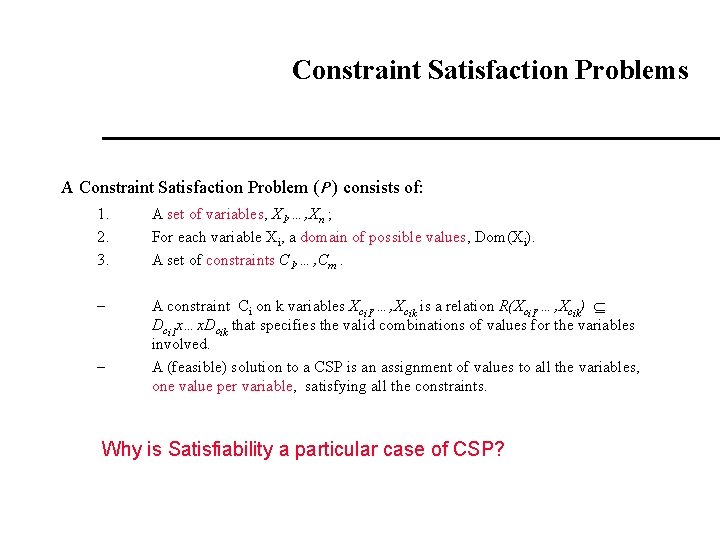
Constraint Satisfaction Problems A Constraint Satisfaction Problem (P ) consists of: 1. 2. 3. A set of variables, X 1, …, Xn ; For each variable Xi, a domain of possible values, Dom(Xi). A set of constraints C 1, …, Cm. – A constraint Ci on k variables Xci 1, …, Xcik is a relation R(Xci 1, …, Xcik) Dci 1 x…x. Dcik that specifies the valid combinations of values for the variables involved. A (feasible) solution to a CSP is an assignment of values to all the variables, one value per variable, satisfying all the constraints. – Why is Satisfiability a particular case of CSP?

A variable V can be assigned a value v (V v) if and only if v Є Dom(V). A consistent set of assignments is a set of assignments {V 1 v 1, …, Vk vk}, such that all the constraints are satisfied, and each of the Vi is unique; A (feasible) solution is a complete consistent set of assignments, i. e. , one consistent set of assignments in which the number of variables in the set is equal to the number of variables in the problem (n).

Any subset of a (feasible) solution is consistent; We might be interested in finding: – Any (feasible) solution – Enumerating or counting all the (feasible) solutions or all optimal solutions – Finding the optimal solution --- i. e. , (feasible) solution(s) that optimize(s) an objective function

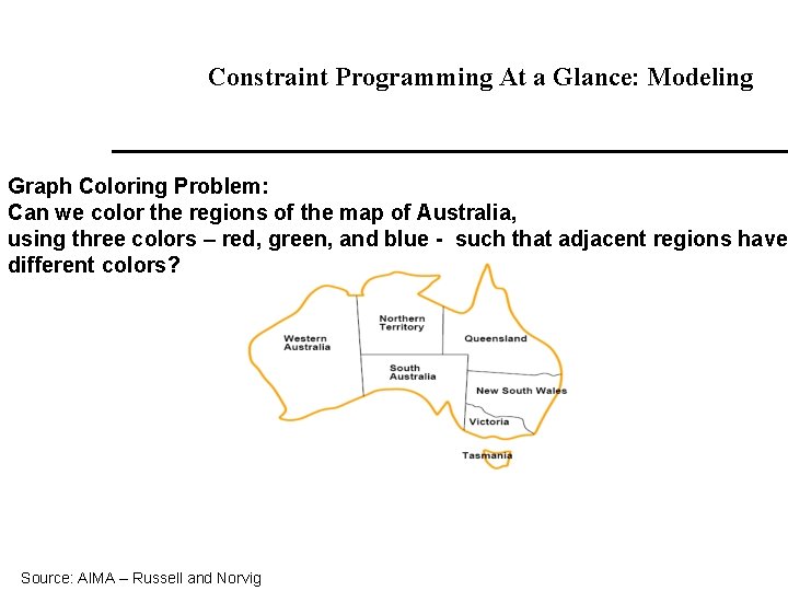
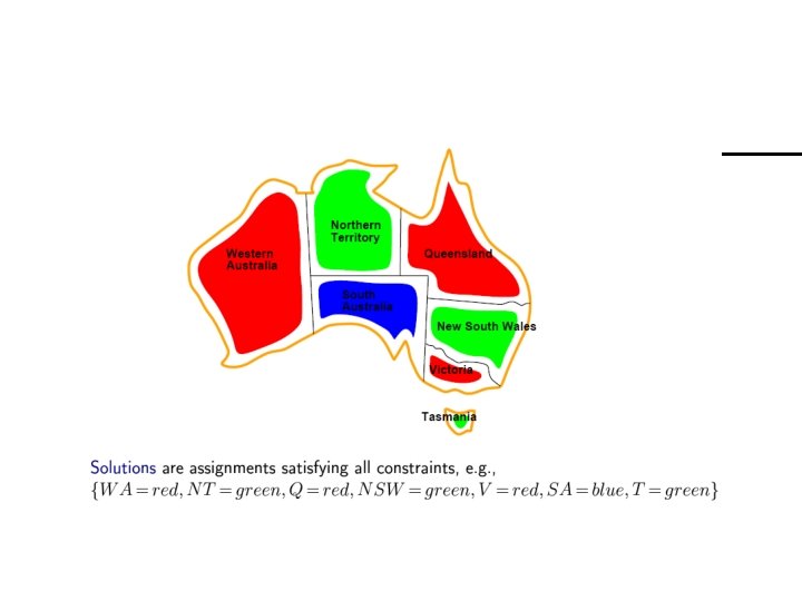
Constraint Programming At a Glance: Modeling Graph Coloring Problem: Can we color the regions of the map of Australia, using three colors – red, green, and blue - such that adjacent regions have different colors? Source: AIMA – Russell and Norvig

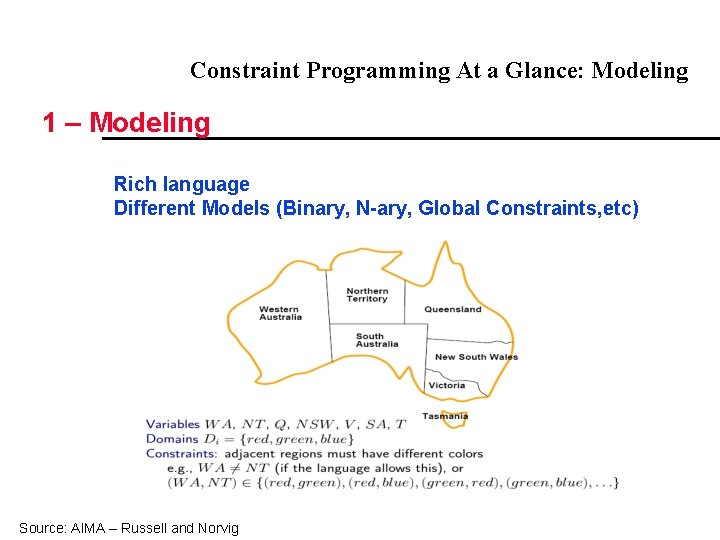
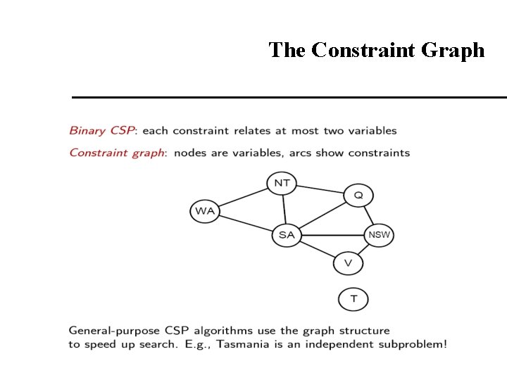
Constraint Programming At a Glance: Modeling 1 – Modeling Rich language Different Models (Binary, N-ary, Global Constraints, etc) Source: AIMA – Russell and Norvig

The Constraint Graph

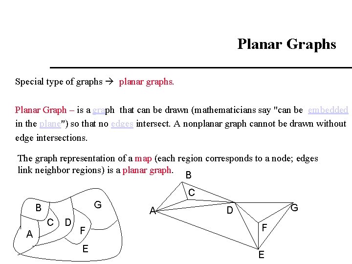
Planar Graphs Special type of graphs planar graphs. Planar Graph – is a graph that can be drawn (mathematicians say "can be embedded in the plane") so that no edges intersect. A nonplanar graph cannot be drawn without edge intersections. The graph representation of a map (each region corresponds to a node; edges link neighbor regions) is a planar graph. B C G B C A D F E A G D F E

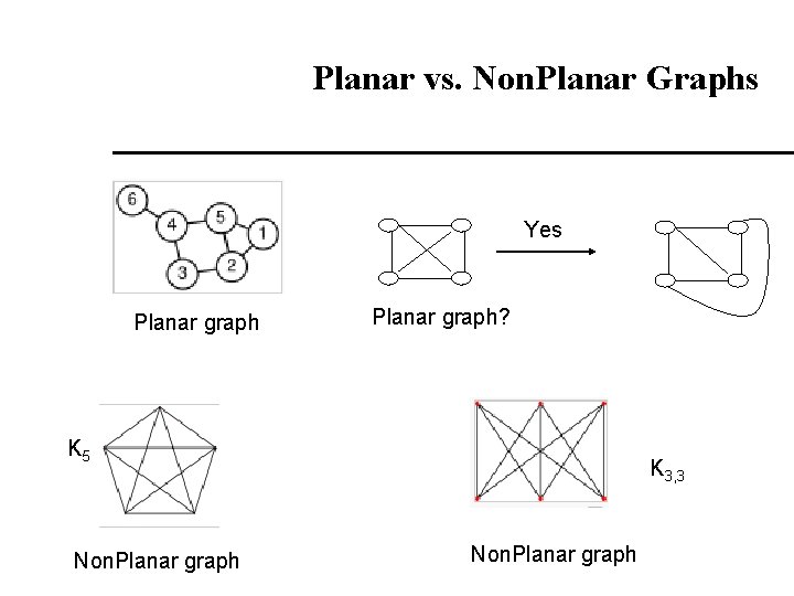
Planar vs. Non. Planar Graphs Yes Planar graph? K 5 Non. Planar graph K 3, 3 Non. Planar graph

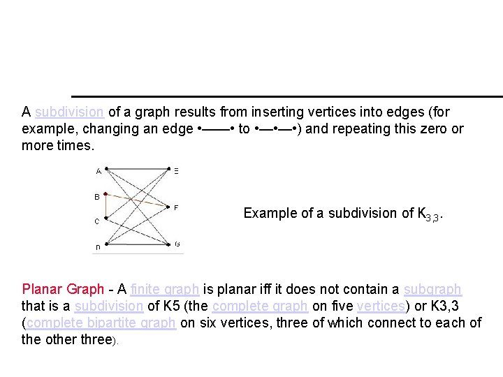
A subdivision of a graph results from inserting vertices into edges (for example, changing an edge • —— • to • — • ) and repeating this zero or more times. Example of a subdivision of K 3, 3. Planar Graph - A finite graph is planar iff it does not contain a subgraph that is a subdivision of K 5 (the complete graph on five vertices) or K 3, 3 (complete bipartite graph on six vertices, three of which connect to each of the other three).

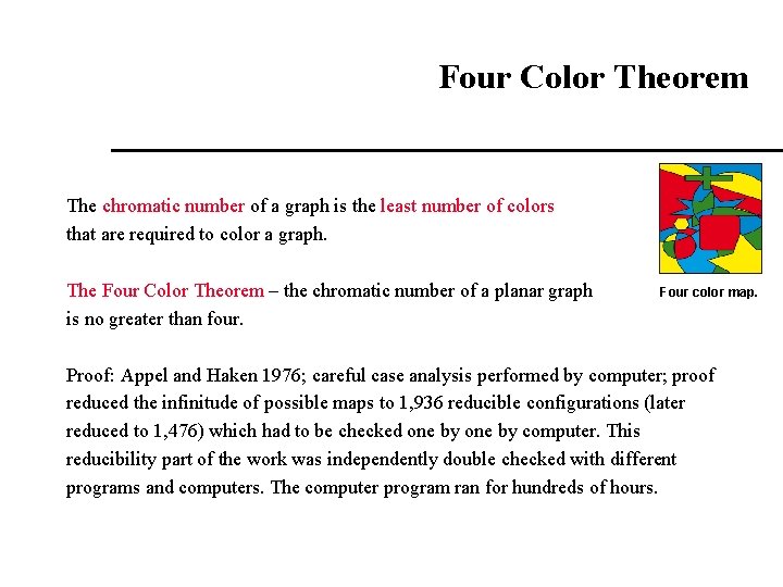
Four Color Theorem The chromatic number of a graph is the least number of colors that are required to color a graph. The Four Color Theorem – the chromatic number of a planar graph is no greater than four. Four color map. Proof: Appel and Haken 1976; careful case analysis performed by computer; proof reduced the infinitude of possible maps to 1, 936 reducible configurations (later reduced to 1, 476) which had to be checked one by computer. This reducibility part of the work was independently double checked with different programs and computers. The computer program ran for hundreds of hours.

Graph Coloring for Arbitrary Graphs Four Color Theorem – only applies to planar graphs; For an arbitrary graph – finding the chromatic number of an arbitrary graph takes exponential time (in the worst-case); even finding an approximation to the chromatic number up to a factor of 2 (i. e. , a bound which is no more than double the chromatic number) is hard – if we found a polynomial time approximation algorithm with less than a factor of 2, then we would also find a polynomial time algorithm for finding the excat chromatic number of the graph.

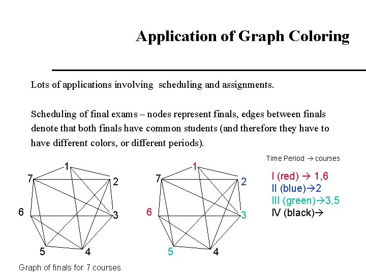
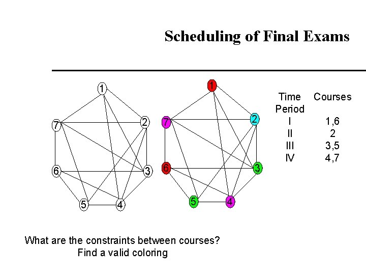
Application of Graph Coloring Lots of applications involving scheduling and assignments. Scheduling of final exams – nodes represent finals, edges between finals denote that both finals have common students (and therefore they have to have different colors, or different periods). 1 1 7 7 2 6 3 5 Time Period courses 4 Graph of finals for 7 courses 2 6 3 5 4 I (red) 1, 6 II (blue) 2 III (green) 3, 5 IV (black)

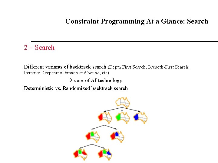
Constraint Programming At a Glance: Search 2 – Search Different variants of backtrack search (Depth First Search; Breadth-First Search; Iterative Deepening; branch and bound, etc) core of AI technology Deterministic vs. Randomized backtrack search

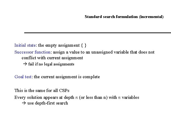
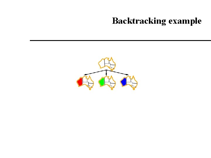
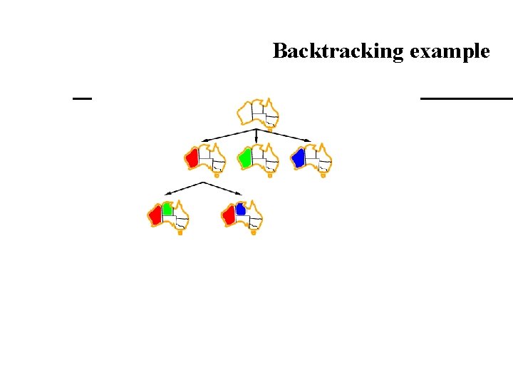
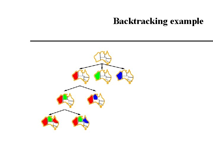
Standard search formulation (incremental) Initial state: the empty assignment { } Successor function: assign a value to an unassigned variable that does not conflict with current assignment fail if no legal assignments Goal test: the current assignment is complete This is the same for all CSPs Every solution appears at depth n (or less than n) with n variables use depth-first search

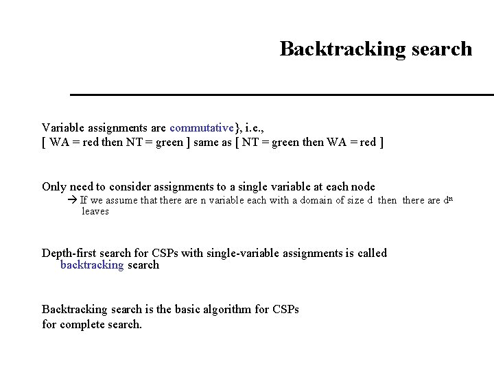
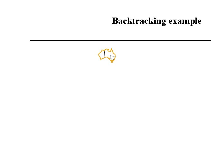
Backtracking search Variable assignments are commutative}, i. e. , [ WA = red then NT = green ] same as [ NT = green then WA = red ] Only need to consider assignments to a single variable at each node If we assume that there are n variable each with a domain of size d then there are dn leaves Depth-first search for CSPs with single-variable assignments is called backtracking search Backtracking search is the basic algorithm for CSPs for complete search.

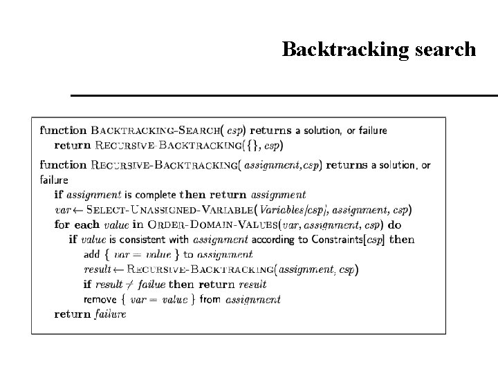
Backtracking search

Backtracking example

Backtracking example

Backtracking example

Backtracking example

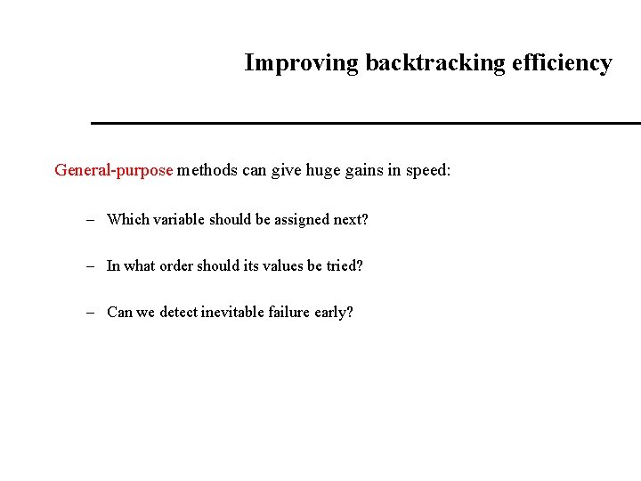
Improving backtracking efficiency General-purpose methods can give huge gains in speed: – Which variable should be assigned next? – In what order should its values be tried? – Can we detect inevitable failure early?

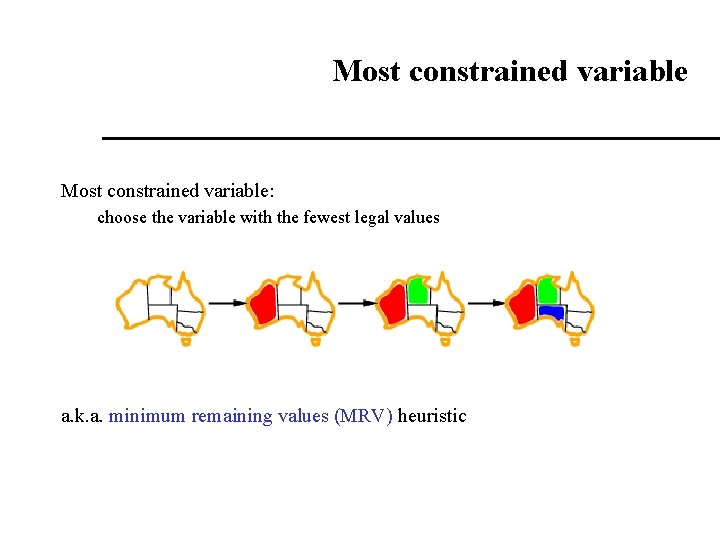
Most constrained variable: choose the variable with the fewest legal values a. k. a. minimum remaining values (MRV) heuristic

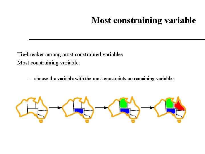
Most constraining variable Tie-breaker among most constrained variables Most constraining variable: – choose the variable with the most constraints on remaining variables

Least constraining value Given a variable, choose the least constraining value: – the one that rules out the fewest values in the remaining variables Combining these heuristics makes 1000 queens feasible

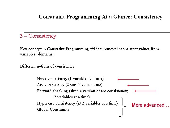
Constraint Programming At a Glance: Consistency 3 – Consistency Key concept in Constraint Programming idea: remove inconsistent values from variables’ domains; Different notions of consistency: Node consistency (1 variable at a time) Arc consistency (2 variables at a time) Forward checking (simple version of arc consistency; 2 variables at a time) Hyper-arc consistency (k>2 variables at a time) More advanced… Global Constraints

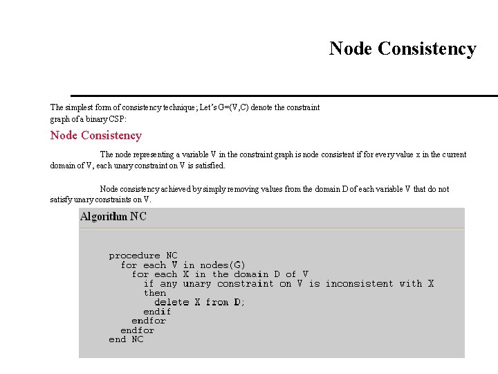
Node Consistency The simplest form of consistency technique; Let’s G=(V, C) denote the constraint graph of a binary CSP: Node Consistency The node representing a variable V in the constraint graph is node consistent if for every value x in the current domain of V, each unary constraint on V is satisfied. Node consistency achieved by simply removing values from the domain D of each variable V that do not satisfy unary constraints on V.

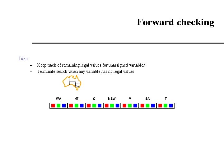
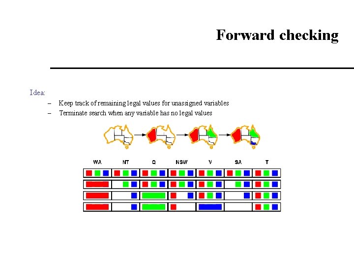
Forward checking Idea: – – Keep track of remaining legal values for unassigned variables Terminate search when any variable has no legal values

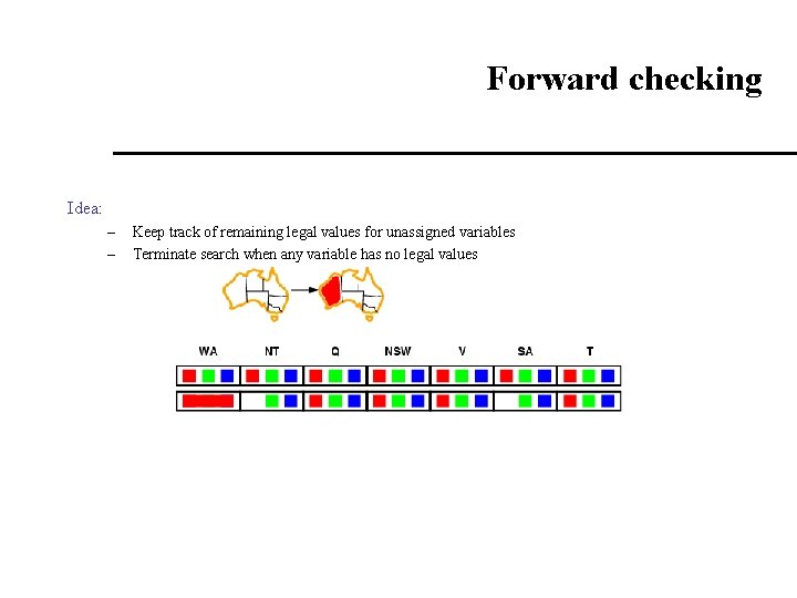
Forward checking Idea: – – Keep track of remaining legal values for unassigned variables Terminate search when any variable has no legal values

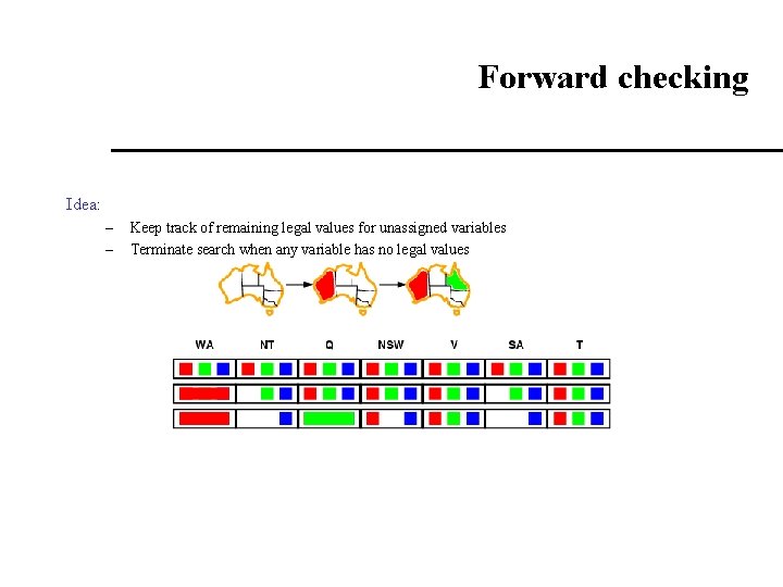
Forward checking Idea: – – Keep track of remaining legal values for unassigned variables Terminate search when any variable has no legal values

Forward checking Idea: – – Keep track of remaining legal values for unassigned variables Terminate search when any variable has no legal values

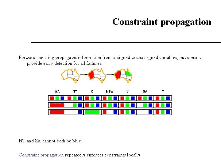
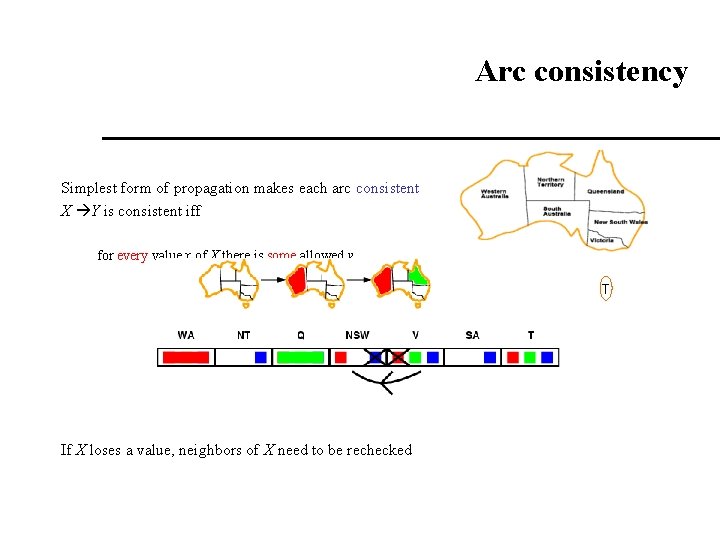
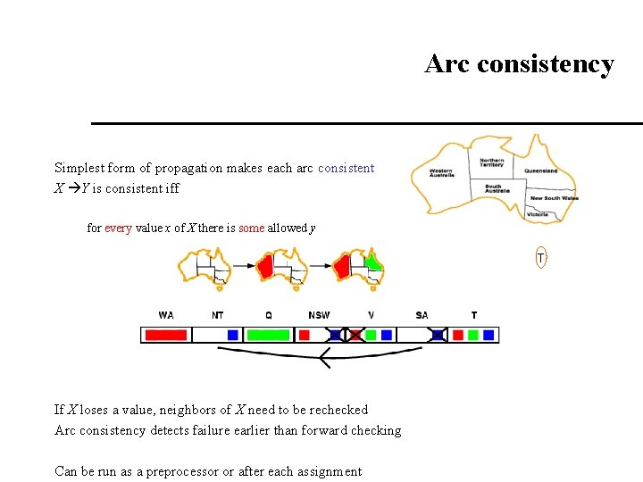
Constraint propagation Forward checking propagates information from assigned to unassigned variables, but doesn't provide early detection for all failures: NT and SA cannot both be blue! Constraint propagation repeatedly enforces constraints locally

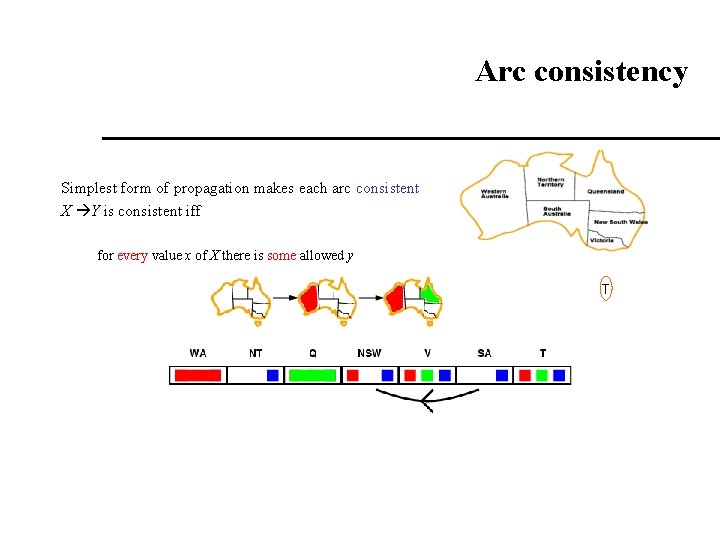
Arc consistency Simplest form of propagation makes each arc consistent X Y is consistent iff for every value x of X there is some allowed y T

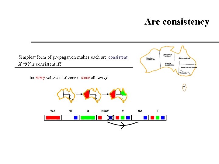
Arc consistency Simplest form of propagation makes each arc consistent X Y is consistent iff for every value x of X there is some allowed y T

Arc consistency Simplest form of propagation makes each arc consistent X Y is consistent iff for every value x of X there is some allowed y T If X loses a value, neighbors of X need to be rechecked

Arc consistency Simplest form of propagation makes each arc consistent X Y is consistent iff for every value x of X there is some allowed y T If X loses a value, neighbors of X need to be rechecked Arc consistency detects failure earlier than forward checking Can be run as a preprocessor or after each assignment

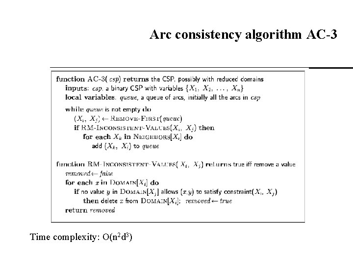
Arc consistency algorithm AC-3 Time complexity: O(n 2 d 3)

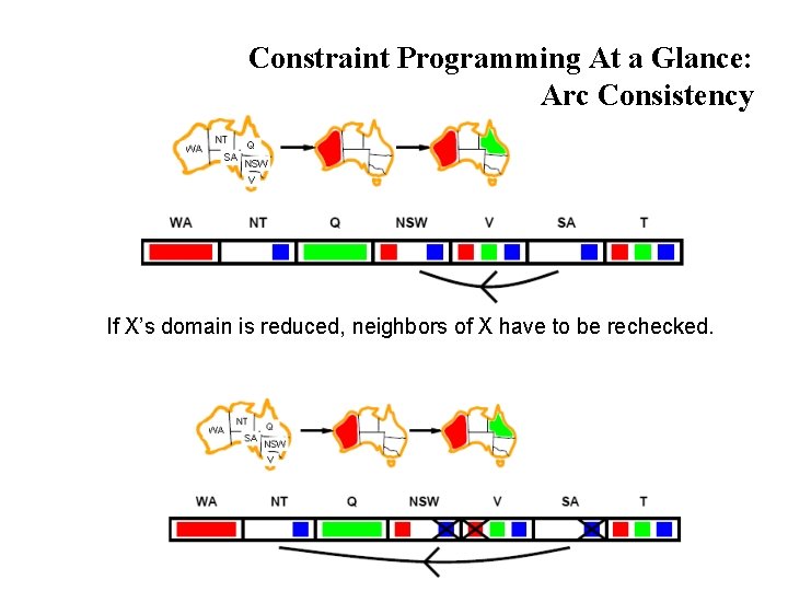
Constraint Programming At a Glance: Arc Consistency If X’s domain is reduced, neighbors of X have to be rechecked.

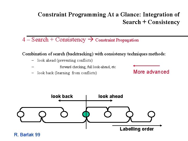
Constraint Programming At a Glance: Integration of Search + Consistency 4 – Search + Consistency Constraint Propagation Combination of search (backtracking) with consistency techniques methods: – look ahead (preventing conflicts) – forward checking, full look-ahead, etc More advanced – look back (learning from conflicts) look back look ahead Labelling order R. Bartak 99

Examples of Applications of Graph Coloring

Scheduling of Final Exams How can the final exams at Cornell be scheduled so that no student nhas two exams at the same time? A vertex correspond to a course; An edge between two vertices denotes that there is at least one common Student in the courses they represent; Each time slot for a final exam is represented by a different color. A coloring of the graph corresponds to a valid schedule of the exams.

Scheduling of Final Exams 1 1 7 2 7 6 3 6 5 4 2 3 5 What are the constraints between courses? Find a valid coloring 4 Time Courses Period I 1, 6 II 2 III 3, 5 IV 4, 7

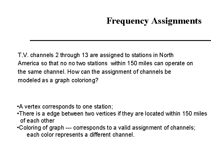
Frequency Assignments T. V. channels 2 through 13 are assigned to stations in North America so that no no two stations within 150 miles can operate on the same channel. How can the assignment of channels be modeled as a graph coloriong? • A vertex corresponds to one station; • There is a edge between two vertices if they are located within 150 miles of each other • Coloring of graph --- corresponds to a valid assignment of channels; each color represents a different channel.

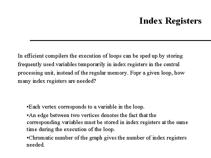
Index Registers In efficient compilers the execution of loops can be sped up by storing frequently used variables temporarily in index registers in the central processing unit, instead of the regular memory. Fopr a given loop, how many index registers are needed? • Each vertex corresponds to a variable in the loop. • An edge between two vertices denotes the fact that the corresponding variables must be stored in index registers at the same time during the execution of the loop. • Chromatic number of the graph gives the number of index registers needed.

Other examples

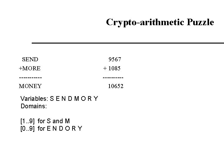
Crypto-arithmetic Puzzle SEND +MORE -----MONEY Variables: S E N D M O R Y Domains: [1. . 9] for S and M [0. . 9] for E N D O R Y 9567 + 1085 -----10652

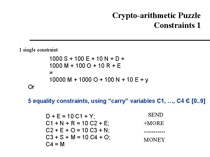
Crypto-arithmetic Puzzle Constraints 1 1 single constraint 1000 S + 100 E + 10 N + D + 1000 M + 100 O + 10 R + E = 10000 M + 1000 O + 100 N + 10 E + y Or 5 equality constraints, using “carry” variables C 1, …, C 4 Є [0. . 9] D + E = 10 C 1 + Y; C 1 + N + R = 10 C 2 + E; C 2 + E + O = 10 C 3 + N; C 3 + S + M = 10 C 4 + O; C 4 = M SEND +MORE -----MONEY

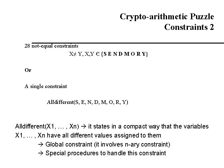
Crypto-arithmetic Puzzle Constraints 2 28 not-equal constraints X≠ Y, X, Y Є {S E N D M O R Y} Or A single constraint Alldifferent(S, E, N, D, M, O, R, Y) Alldifferent(X 1, … , Xn) it states in a compact way that the variables X 1, … , Xn have all different values assigned to them Global constraint (it involves n-ary constraint) Special procedures to handle this constraint

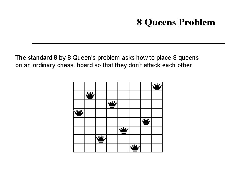
8 Queens Problem The standard 8 by 8 Queen's problem asks how to place 8 queens on an ordinary chess board so that they don’t attack each other

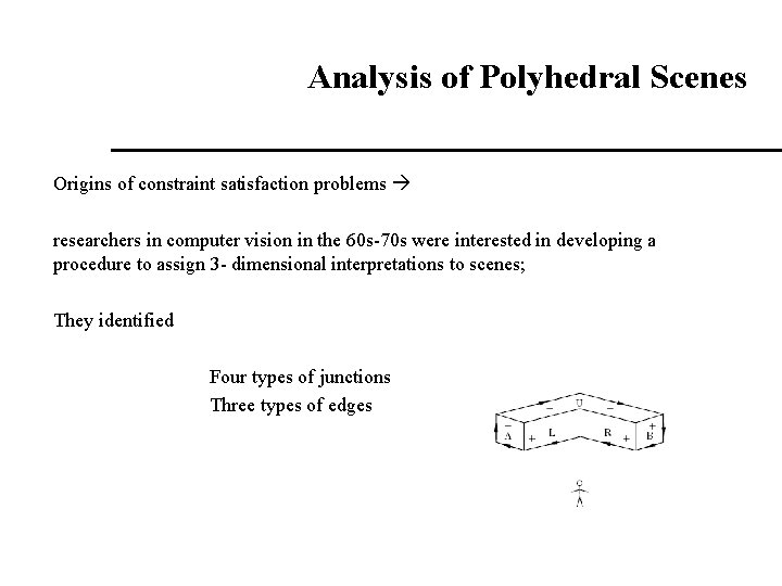
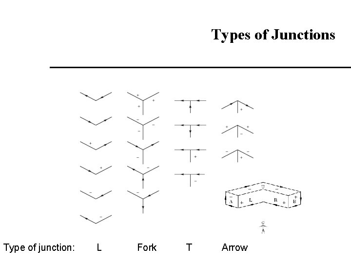
Analysis of Polyhedral Scenes Origins of constraint satisfaction problems researchers in computer vision in the 60 s-70 s were interested in developing a procedure to assign 3 - dimensional interpretations to scenes; They identified Four types of junctions Three types of edges

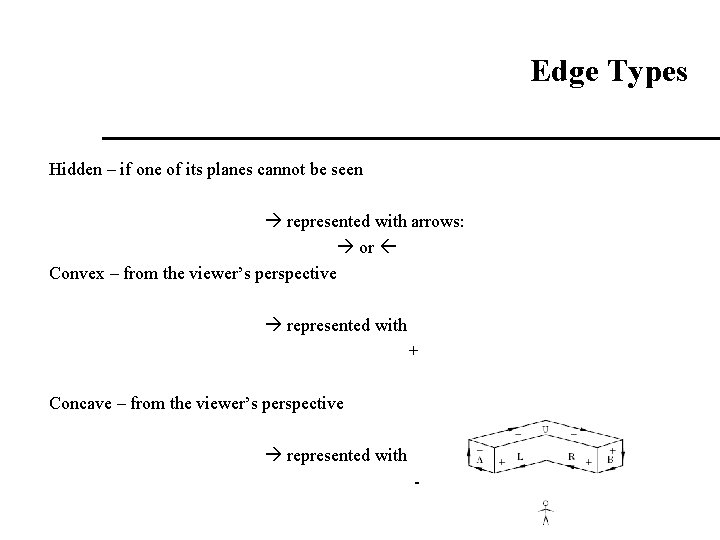
Edge Types Hidden – if one of its planes cannot be seen represented with arrows: or Convex – from the viewer’s perspective represented with + Concave – from the viewer’s perspective represented with -

Types of Junctions Type of junction: L Fork T Arrow

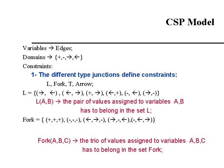
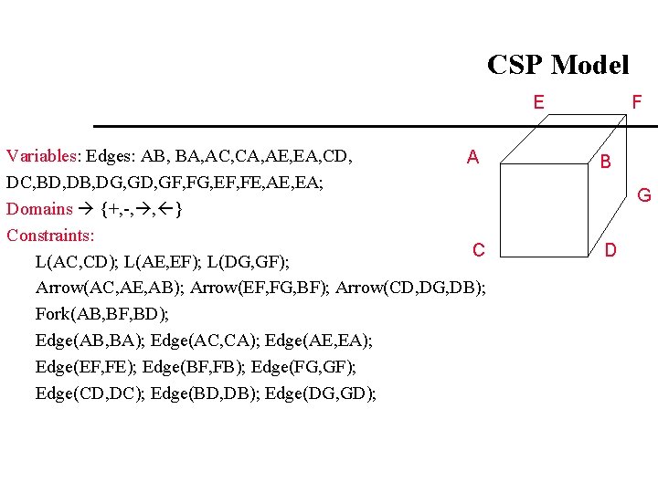
CSP Model Variables Edges; Domains {+, -, , } Constraints: 1 - The different type junctions define constraints: L, Fork, T, Arrow; L = {( , ) , ( , ), (+, ), ( , +), (-, ), ( , -)} L(A, B) the pair of values assigned to variables A, B has to belong in the set L; Fork = { (+, +, +), (-, -, -), ( , -, ), (-, , )} Fork(A, B, C) the trio of values assigned to variables A, B, C has to belong in the set Fork;

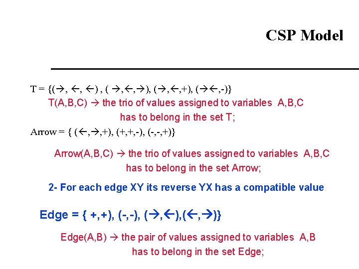
CSP Model T = {( , , ) , ( , , ), ( , , +), ( , -)} T(A, B, C) the trio of values assigned to variables A, B, C has to belong in the set T; Arrow = { ( , , +), (+, +, -), (-, -, +)} Arrow(A, B, C) the trio of values assigned to variables A, B, C has to belong in the set Arrow; 2 - For each edge XY its reverse YX has a compatible value Edge = { +, +), (-, -), ( , )} Edge(A, B) the pair of values assigned to variables A, B has to belong in the set Edge;

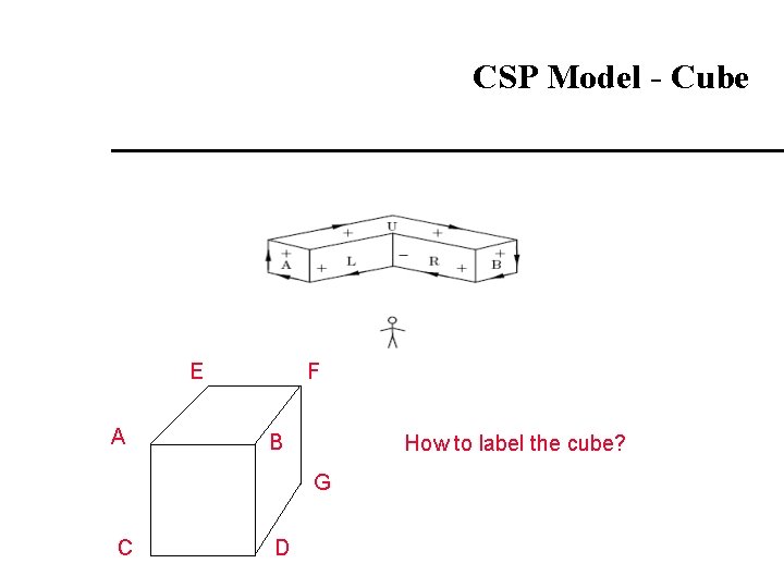
CSP Model - Cube E A F B How to label the cube? G C D

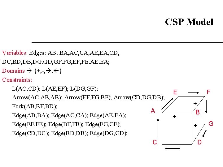
CSP Model E Variables: Edges: AB, BA, AC, CA, AE, EA, CD, A DC, BD, DB, DG, GD, GF, FG, EF, FE, AE, EA; Domains {+, -, , } Constraints: C L(AC, CD); L(AE, EF); L(DG, GF); Arrow(AC, AE, AB); Arrow(EF, FG, BF); Arrow(CD, DG, DB); Fork(AB, BF, BD); Edge(AB, BA); Edge(AC, CA); Edge(AE, EA); Edge(EF, FE); Edge(BF, FB); Edge(FG, GF); Edge(CD, DC); Edge(BD, DB); Edge(DG, GD); F B G D

CSP Model Variables: Edges: AB, BA, AC, CA, AE, EA, CD, DC, BD, DB, DG, GD, GF, FG, EF, FE, AE, EA; Domains {+, -, , } Constraints: L(AC, CD); L(AE, EF); L(DG, GF); Arrow(AC, AE, AB); Arrow(EF, FG, BF); Arrow(CD, DG, DB); Fork(AB, BF, BD); A Edge(AB, BA); Edge(AC, CA); Edge(AE, EA); Edge(EF, FE); Edge(BF, FB); Edge(FG, GF); Edge(CD, DC); Edge(BD, DB); Edge(DG, GD); C E + F + B G + D

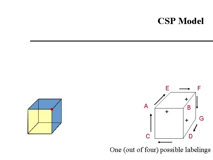
CSP Model E A + F + B G + C D One (out of four) possible labelings

Escher: Waterfall, 1961

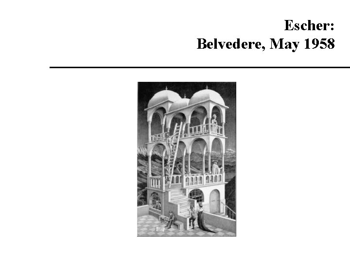
Escher: Belvedere, May 1958

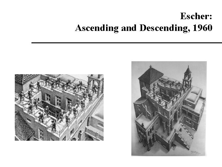
Escher: Ascending and Descending, 1960

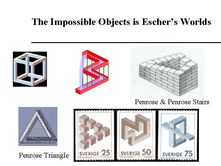
The Impossible Objects is Escher’s Worlds Penrose & Penrose Stairs Penrose Triangle

Impossible Objects: No labeling!

Real-World Applications Hardware and Software Configuration Hardware and Software Verification Timetabling Sport Scheduling Floor-Planning Car Sequencing Transporation scheduling

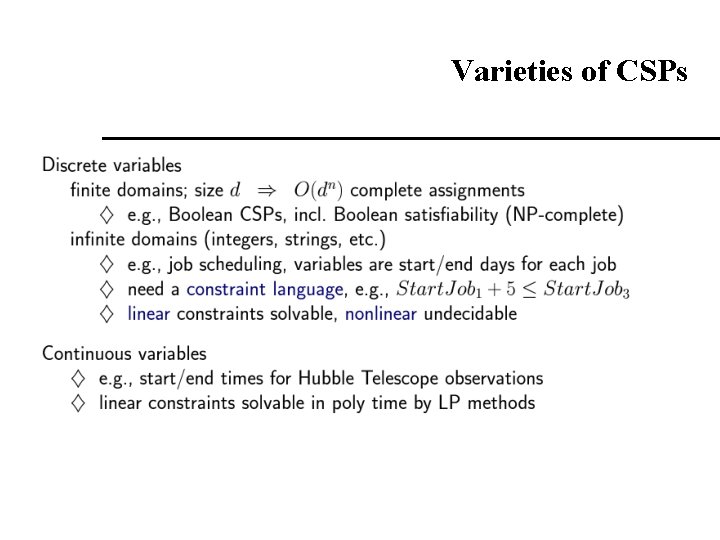
Varieties of CSPs

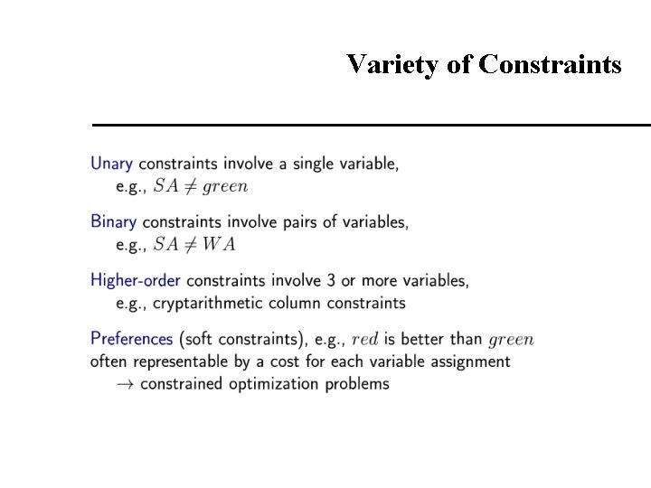
Variety of Constraints

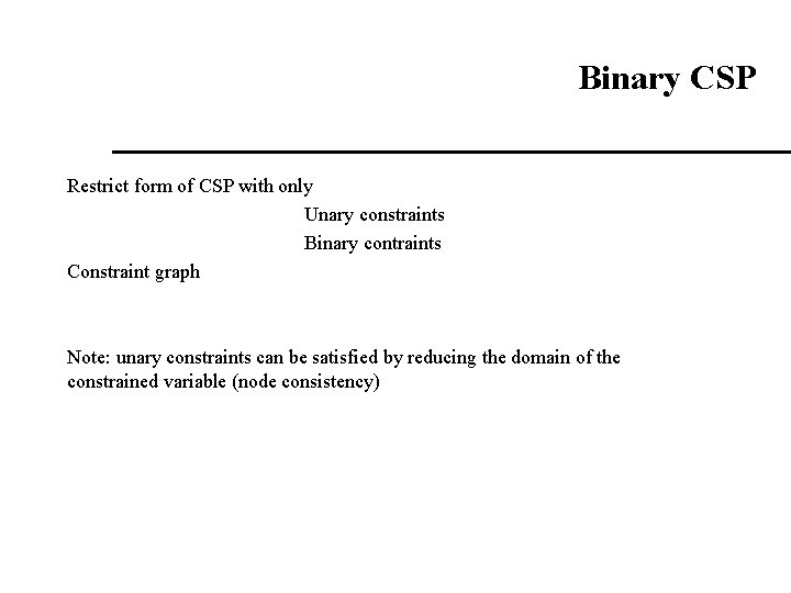
Binary CSP Restrict form of CSP with only Unary constraints Binary contraints Constraint graph Note: unary constraints can be satisfied by reducing the domain of the constrained variable (node consistency)

Further reading Algorithms for Constraint Satisfaction Problems: A Survey, Vipin Kumar, in AI Magazine 13(1): 32 -44, 1992 (available online).