Inventory Management LO 20 1 Explain how inventory

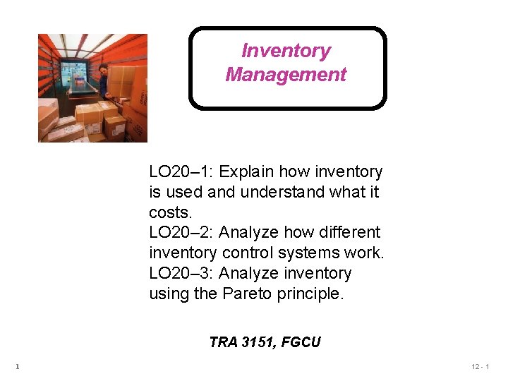
Inventory Management LO 20– 1: Explain how inventory is used and understand what it costs. LO 20– 2: Analyze how different inventory control systems work. LO 20– 3: Analyze inventory using the Pareto principle. TRA 3151, FGCU 1 12 - 1

Outline u The Importance of Inventory u Functions of Inventory u Types of Inventory u Managing Inventory u ABC Analysis u Inventory Models u Independent vs. Dependent Demand u Holding, Ordering, and Setup Costs 12 - 2

Outline – Continued u Inventory Models for Independent Demand u The Basic Economic Order Quantity (EOQ) Model u Minimizing Costs u Reorder Points u Probabilistic Models and Safety Stock © 2011 Pearson Education, Inc. publishing as Prentice Hall 12 - 3

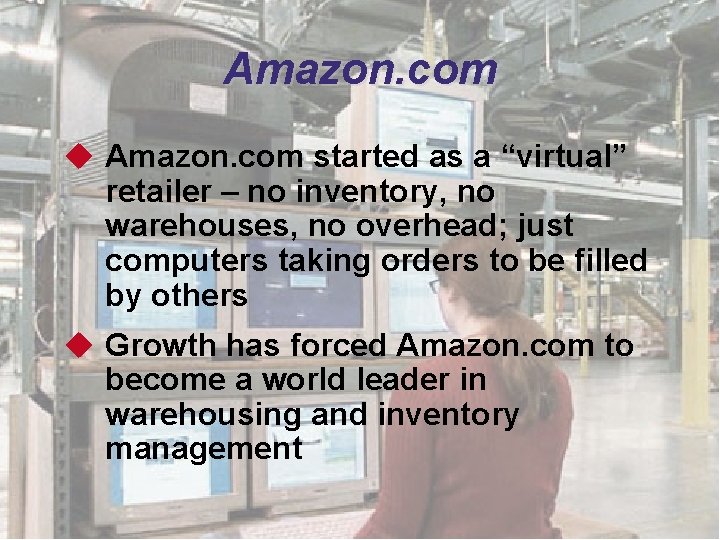
Amazon. com u Amazon. com started as a “virtual” retailer – no inventory, no warehouses, no overhead; just computers taking orders to be filled by others u Growth has forced Amazon. com to become a world leader in warehousing and inventory management © 2011 Pearson Education, Inc. publishing as Prentice Hall 12 - 4

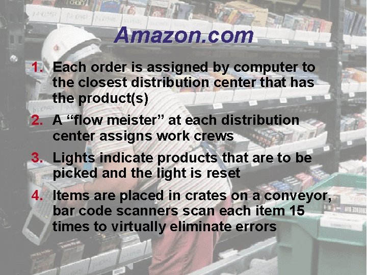
Amazon. com 1. Each order is assigned by computer to the closest distribution center that has the product(s) 2. A “flow meister” at each distribution center assigns work crews 3. Lights indicate products that are to be picked and the light is reset 4. Items are placed in crates on a conveyor, bar code scanners scan each item 15 times to virtually eliminate errors © 2011 Pearson Education, Inc. publishing as Prentice Hall 12 - 5

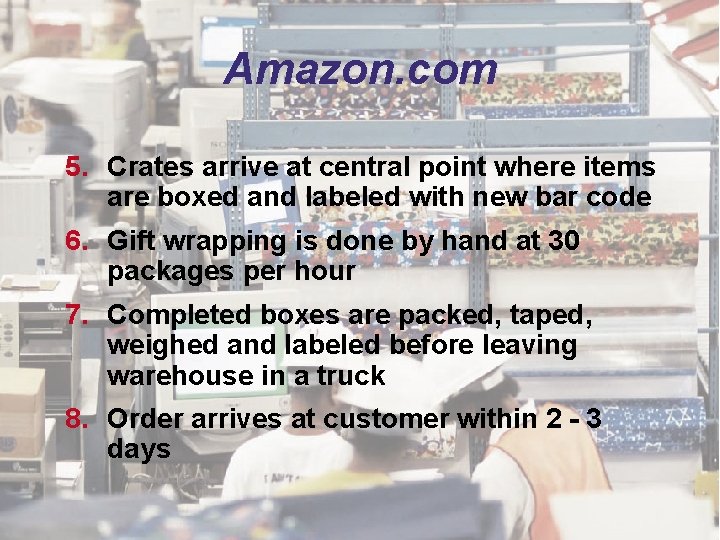
Amazon. com 5. Crates arrive at central point where items are boxed and labeled with new bar code 6. Gift wrapping is done by hand at 30 packages per hour 7. Completed boxes are packed, taped, weighed and labeled before leaving warehouse in a truck 8. Order arrives at customer within 2 - 3 days © 2011 Pearson Education, Inc. publishing as Prentice Hall 12 - 6

Importance of Inventory u One of the most expensive assets of many companies representing as much as 50% of total invested capital u Operations managers must balance inventory investment and customer service © 2011 Pearson Education, Inc. publishing as Prentice Hall 12 - 7

Inventory u Inventory can be visualized as stacks of money sitting on forklifts, on shelves, and in trucks and planes while in transit. u For many businesses, inventory is the largest asset on the balance sheet at any given time. u Inventory can be difficult to convert back into cash. u It is a good idea to try to get your inventory down as far as possible. u The average cost of inventory in the United States is 30 to 35 percent of its value. 20 -8 12 - 8

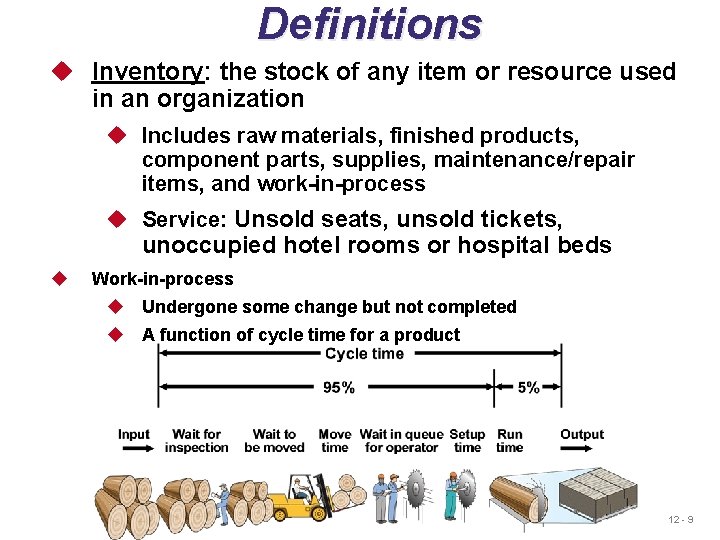
Definitions u Inventory: the stock of any item or resource used in an organization u Includes raw materials, finished products, component parts, supplies, maintenance/repair items, and work-in-process u Service: Unsold seats, unsold tickets, unoccupied hotel rooms or hospital beds u Work-in-process u Undergone some change but not completed u A function of cycle time for a product 12 - 9

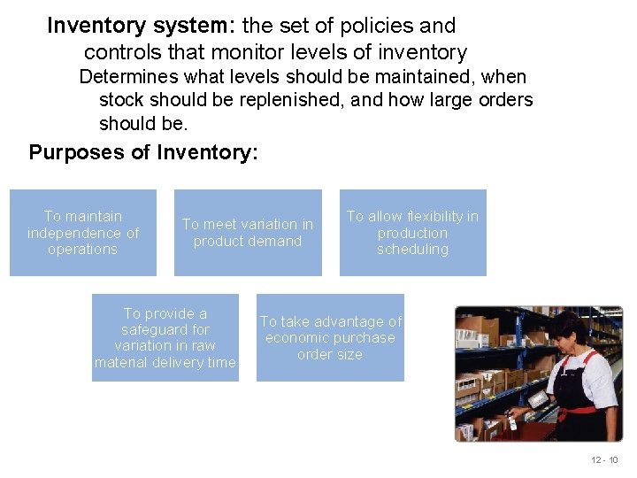
Inventory system: the set of policies and controls that monitor levels of inventory Determines what levels should be maintained, when stock should be replenished, and how large orders should be. Purposes of Inventory: To maintain independence of operations To meet variation in product demand To provide a safeguard for variation in raw material delivery time To allow flexibility in production scheduling To take advantage of economic purchase order size 12 - 10

Inventory Management The objective of inventory management is to strike a balance between inventory investment and customer service © 2011 Pearson Education, Inc. publishing as Prentice Hall 12 - 11

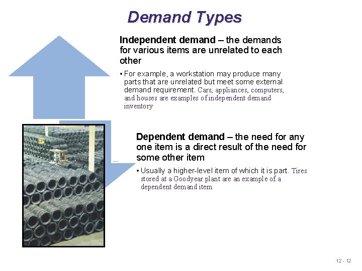
Demand Types Independent demand – the demands for various items are unrelated to each other • For example, a workstation may produce many parts that are unrelated but meet some external demand requirement. Cars, appliances, computers, and houses are examples of independent demand inventory Dependent demand – the need for any one item is a direct result of the need for some other item • Usually a higher-level item of which it is part. Tires stored at a Goodyear plant are an example of a dependent demand item 12 - 12

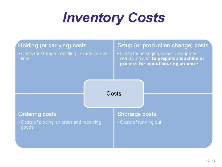
Inventory Costs Holding (or carrying) costs Setup (or production change) costs • Costs for storage, handling, insurance over time • Costs for arranging specific equipment setups, so cost to prepare a machine or process for manufacturing an order Costs Ordering costs Shortage costs • Costs of placing an order and receiving goods • Costs of running out 12 - 13

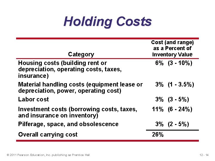
Holding Costs Category Housing costs (building rent or depreciation, operating costs, taxes, insurance) Material handling costs (equipment lease or depreciation, power, operating cost) Labor cost Cost (and range) as a Percent of Inventory Value 6% (3 - 10%) 3% (1 - 3. 5%) 3% (3 - 5%) Investment costs (borrowing costs, taxes, and insurance on inventory) Pilferage, space, and obsolescence 11% (6 - 24%) Overall carrying cost 26% © 2011 Pearson Education, Inc. publishing as Prentice Hall 3% (2 - 5%) 12 - 14

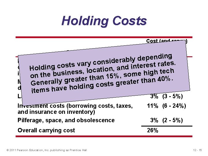
Holding Costs Cost (and range) as a Percent of Inventory Value Category g n i d n e p e d rably Housing costs (building rent or 6% (3 - 10%) e d i s n o c y r tes. a a v r t s s e r o e c t n g i depreciation, operating costs, taxes, n , and Holdi n o i t a c h o l c , e s t s h e g n i i h insurance) s u e , som % on the b 5 1 n a h t r %. e 0 t 4 a e n r a g h t y l r l Material handling costs (equipment lease or 3% (1 - 3. 5%) e a t r grea Gene s t s o c g n i d hol depreciation, power, operating cost) items have Labor cost 3% (3 - 5%) Investment costs (borrowing costs, taxes, and insurance on inventory) Pilferage, space, and obsolescence 11% (6 - 24%) Overall carrying cost 26% © 2011 Pearson Education, Inc. publishing as Prentice Hall 3% (2 - 5%) 12 - 15

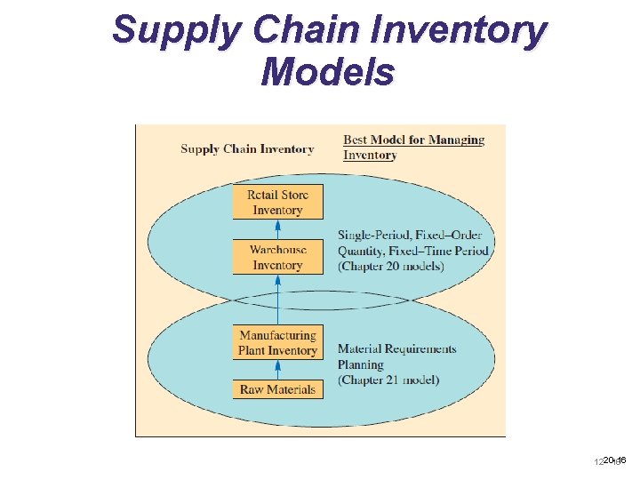
Supply Chain Inventory Models 20 -16 12 - 16

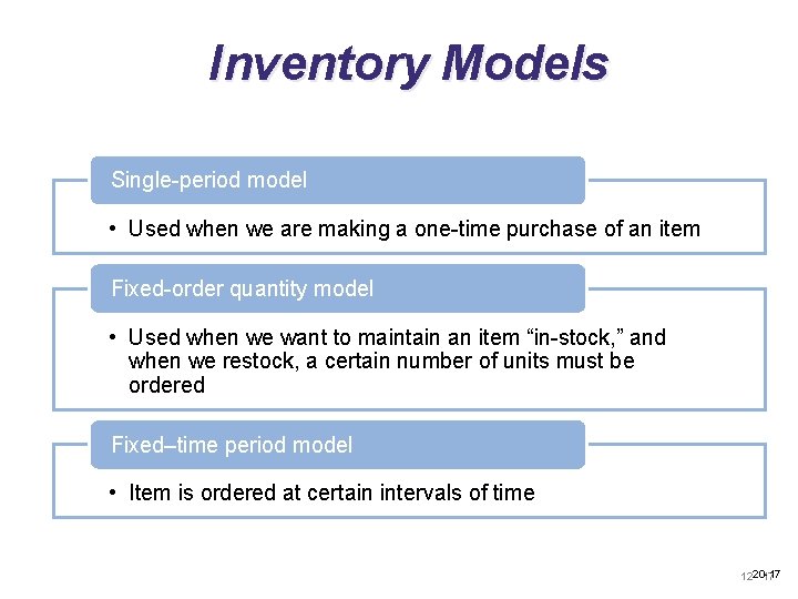
Inventory Models Single-period model • Used when we are making a one-time purchase of an item Fixed-order quantity model • Used when we want to maintain an item “in-stock, ” and when we restock, a certain number of units must be ordered Fixed–time period model • Item is ordered at certain intervals of time 20 -17 12 - 17

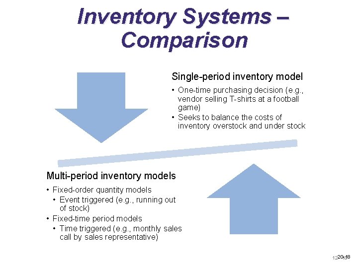
Inventory Systems – Comparison Single-period inventory model • One-time purchasing decision (e. g. , vendor selling T-shirts at a football game) • Seeks to balance the costs of inventory overstock and under stock Multi-period inventory models • Fixed-order quantity models • Event triggered (e. g. , running out of stock) • Fixed-time period models • Time triggered (e. g. , monthly sales call by sales representative) 20 -18 12 - 18

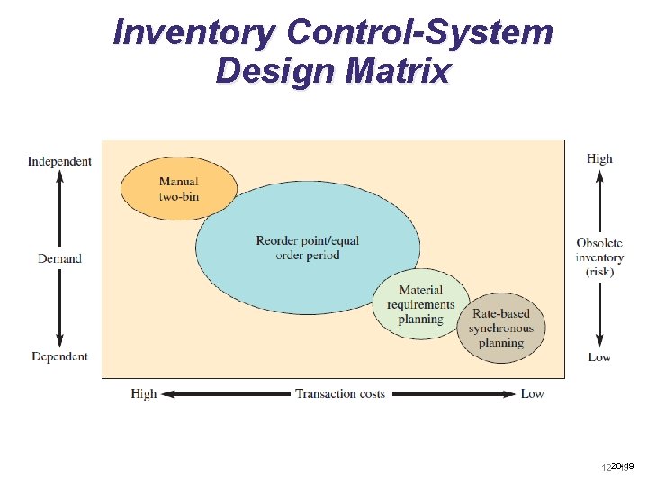
Inventory Control-System Design Matrix 20 -19 12 - 19

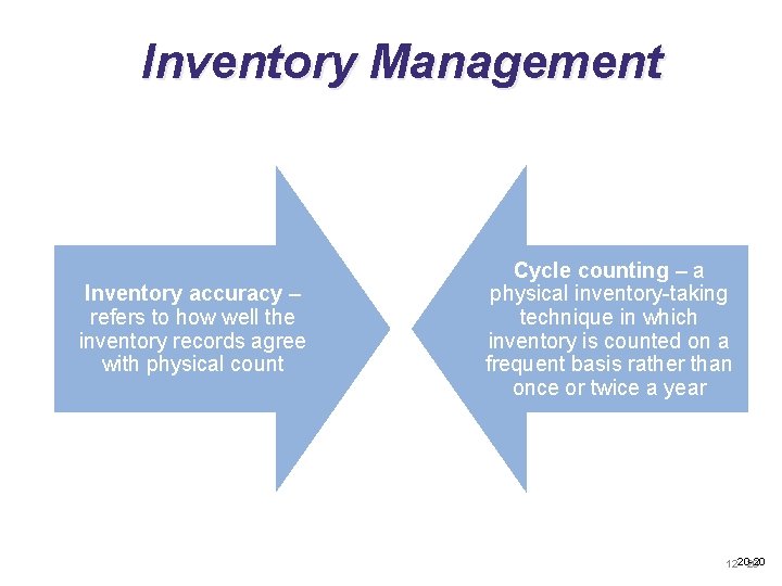
Inventory Management Inventory accuracy – refers to how well the inventory records agree with physical count Cycle counting – a physical inventory-taking technique in which inventory is counted on a frequent basis rather than once or twice a year 20 -20 12 - 20

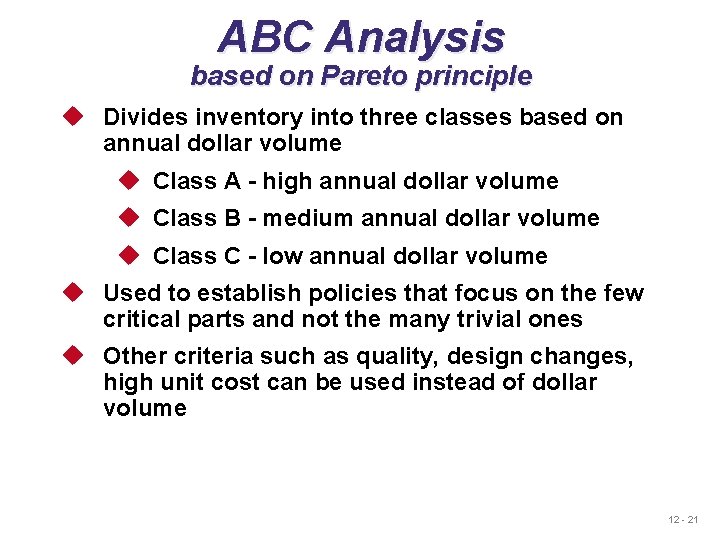
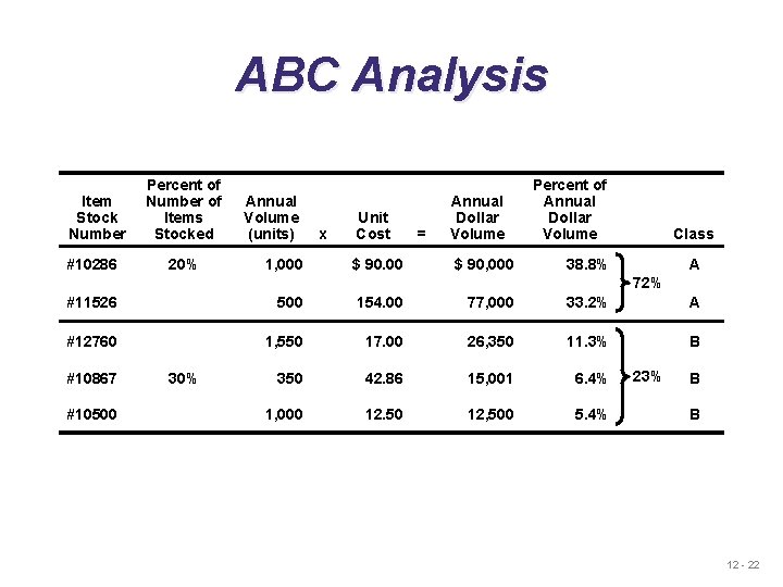
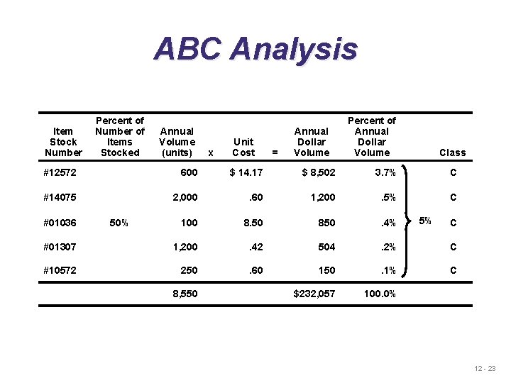
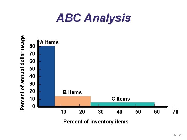
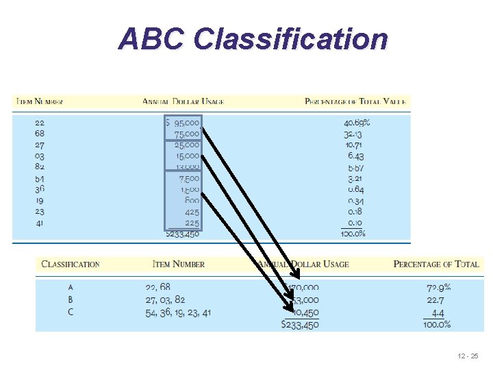
ABC Analysis based on Pareto principle u Divides inventory into three classes based on annual dollar volume u Class A - high annual dollar volume u Class B - medium annual dollar volume u Class C - low annual dollar volume u Used to establish policies that focus on the few critical parts and not the many trivial ones u Other criteria such as quality, design changes, high unit cost can be used instead of dollar volume 12 - 21

ABC Analysis Item Stock Number #10286 Percent of Number of Items Stocked 20% Annual Volume (units) 1, 000 x Unit Cost $ 90. 00 = Annual Dollar Volume $ 90, 000 Percent of Annual Dollar Volume Class 38. 8% A 72% #11526 500 154. 00 77, 000 33. 2% A #12760 1, 550 17. 00 26, 350 11. 3% B 350 42. 86 15, 001 6. 4% 1, 000 12. 50 12, 500 5. 4% #10867 #10500 30% 23% B B 12 - 22

ABC Analysis Item Stock Number Percent of Number of Items Stocked Annual Volume (units) x Unit Cost = Annual Dollar Volume Percent of Annual Dollar Volume Class #12572 600 $ 14. 17 $ 8, 502 3. 7% C #14075 2, 000 . 60 1, 200 . 5% C 100 8. 50 850 . 4% #01307 1, 200 . 42 504 . 2% C #10572 250 . 60 150 . 1% C $232, 057 100. 0% #01036 50% 8, 550 5% C 12 - 23

Percent of annual dollar usage ABC Analysis A Items 80 – 70 – 60 – 50 – 40 – 30 – 20 – B Items 10 – | | 0 – 10 20 C Items | | | 30 40 50 60 70 Percent of inventory items 12 - 24

ABC Classification 12 - 25

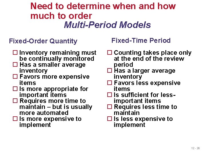
Need to determine when and how much to order Multi-Period Models Fixed-Order Quantity Inventory remaining must be continually monitored Has a smaller average inventory Favors more expensive items Is more appropriate for important items Requires more time to maintain – but is usually more automated Is more expensive to implement Fixed-Time Period Counting takes place only at the end of the review period Has a larger average inventory Favors less expensive items Is sufficient for lessimportant items Requires less time to maintain Is less expensive to implement 12 - 26

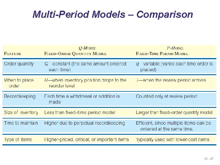
Multi-Period Models – Comparison 12 - 27

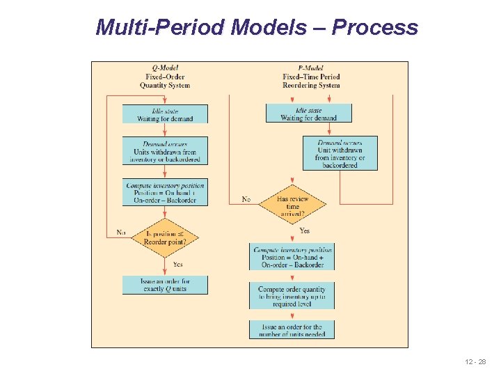
Multi-Period Models – Process 12 - 28

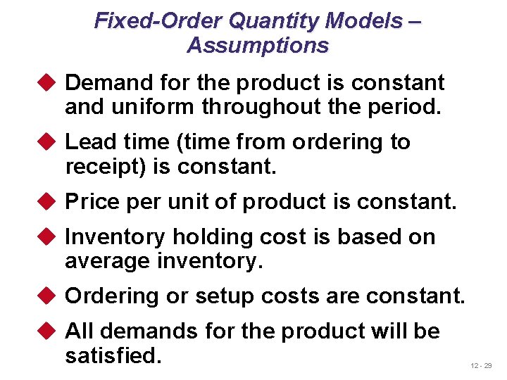
Fixed-Order Quantity Models – Assumptions u Demand for the product is constant and uniform throughout the period. u Lead time (time from ordering to receipt) is constant. u Price per unit of product is constant. u Inventory holding cost is based on average inventory. u Ordering or setup costs are constant. u All demands for the product will be satisfied. 12 - 29

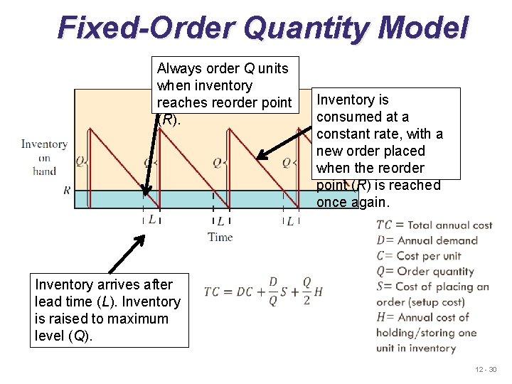
Fixed-Order Quantity Model Always order Q units when inventory reaches reorder point (R). Inventory is consumed at a constant rate, with a new order placed when the reorder point (R) is reached once again. Inventory arrives after lead time (L). Inventory is raised to maximum level (Q). 12 - 30

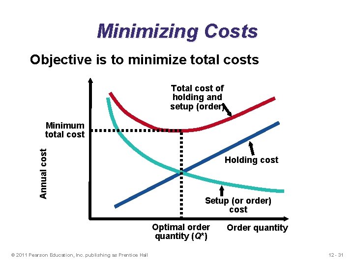
Minimizing Costs Objective is to minimize total costs Total cost of holding and setup (order) Annual cost Minimum total cost Holding cost Setup (or order) cost Optimal order quantity (Q*) © 2011 Pearson Education, Inc. publishing as Prentice Hall Order quantity 12 - 31

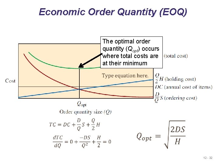
Economic Order Quantity (EOQ) The optimal order quantity (Qopt) occurs where total costs are at their minimum 12 - 32

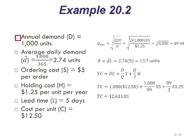
Example 20. 2 12 - 33

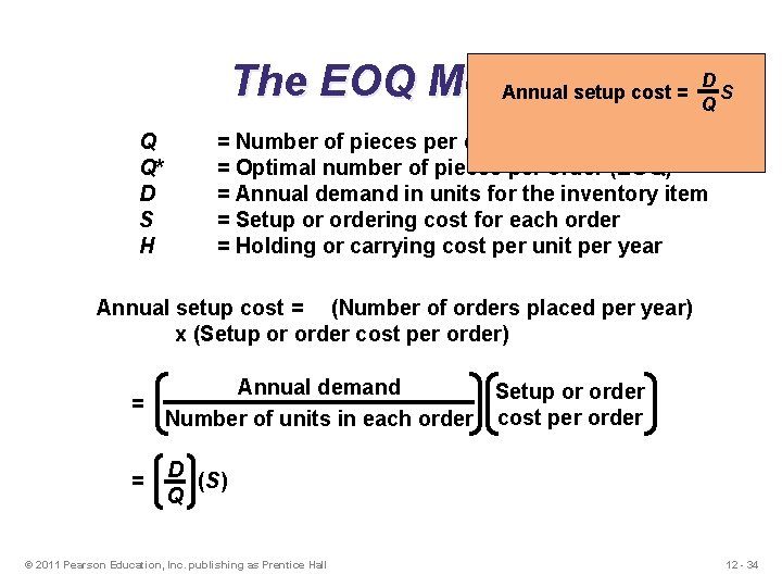
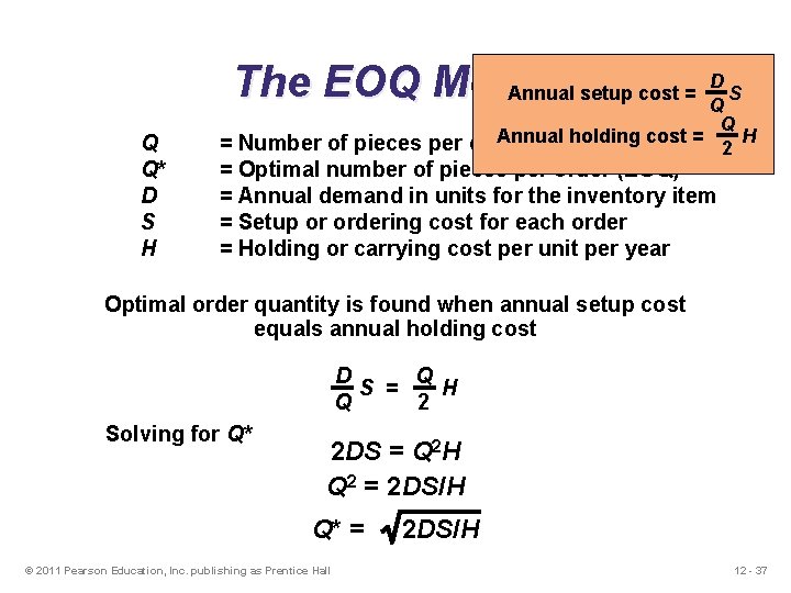
D The EOQ Model Annual setup cost = S Q Q Q* D S H = Number of pieces per order = Optimal number of pieces per order (EOQ) = Annual demand in units for the inventory item = Setup or ordering cost for each order = Holding or carrying cost per unit per year Annual setup cost = (Number of orders placed per year) x (Setup or order cost per order) Annual demand Setup or order = Number of units in each order cost per order D = (S) Q © 2011 Pearson Education, Inc. publishing as Prentice Hall 12 - 34

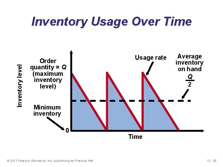
Inventory level Inventory Usage Over Time Order quantity = Q (maximum inventory level) Usage rate Average inventory on hand Q 2 Minimum inventory 0 © 2011 Pearson Education, Inc. publishing as Prentice Hall Time 12 - 35

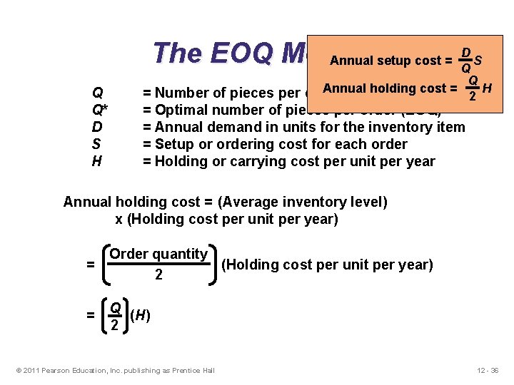
D The EOQ Model Annual setup cost = S Q Q Q* D S H Q Annual holding cost = H = Number of pieces per order 2 = Optimal number of pieces per order (EOQ) = Annual demand in units for the inventory item = Setup or ordering cost for each order = Holding or carrying cost per unit per year Annual holding cost = (Average inventory level) x (Holding cost per unit per year) Order quantity = (Holding cost per unit per year) 2 Q = (H) 2 © 2011 Pearson Education, Inc. publishing as Prentice Hall 12 - 36

D The EOQ Model Annual setup cost = S Q Q Q* D S H Q Annual holding cost = H = Number of pieces per order 2 = Optimal number of pieces per order (EOQ) = Annual demand in units for the inventory item = Setup or ordering cost for each order = Holding or carrying cost per unit per year Optimal order quantity is found when annual setup cost equals annual holding cost D Q S = H Q 2 Solving for Q* 2 DS = Q 2 H Q 2 = 2 DS/H Q* = 2 DS/H © 2011 Pearson Education, Inc. publishing as Prentice Hall 12 - 37

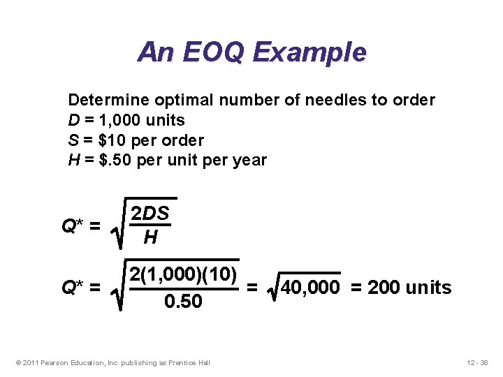
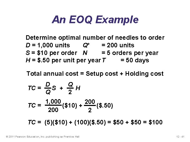
An EOQ Example Determine optimal number of needles to order D = 1, 000 units S = $10 per order H = $. 50 per unit per year Q* = 2 DS H Q* = 2(1, 000)(10) = 40, 000 = 200 units 0. 50 © 2011 Pearson Education, Inc. publishing as Prentice Hall 12 - 38

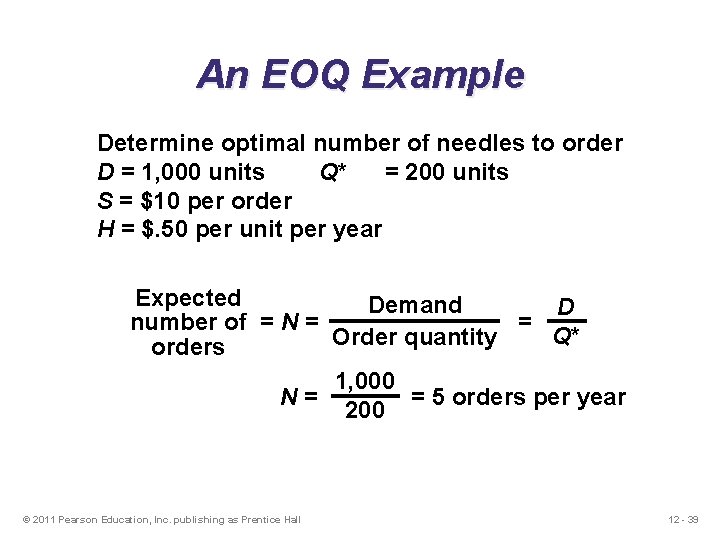
An EOQ Example Determine optimal number of needles to order D = 1, 000 units Q* = 200 units S = $10 per order H = $. 50 per unit per year Expected Demand D number of = N = = Q* Order quantity orders 1, 000 N = = 5 orders per year 200 © 2011 Pearson Education, Inc. publishing as Prentice Hall 12 - 39

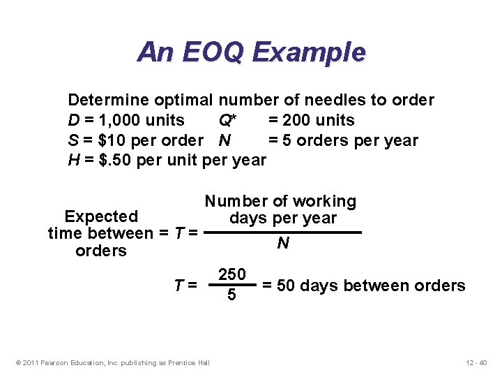
An EOQ Example Determine optimal number of needles to order D = 1, 000 units Q* = 200 units S = $10 per order N = 5 orders per year H = $. 50 per unit per year Expected time between = T = orders Number of working days per year N 250 T = = 50 days between orders 5 © 2011 Pearson Education, Inc. publishing as Prentice Hall 12 - 40

An EOQ Example Determine optimal number of needles to order D = 1, 000 units Q* = 200 units S = $10 per order N = 5 orders per year H = $. 50 per unit per year. T = 50 days Total annual cost = Setup cost + Holding cost Q D TC = S + H 2 Q 1, 000 200 TC = ($10) + ($. 50) 200 2 TC = (5)($10) + (100)($. 50) = $50 + $50 = $100 © 2011 Pearson Education, Inc. publishing as Prentice Hall 12 - 41

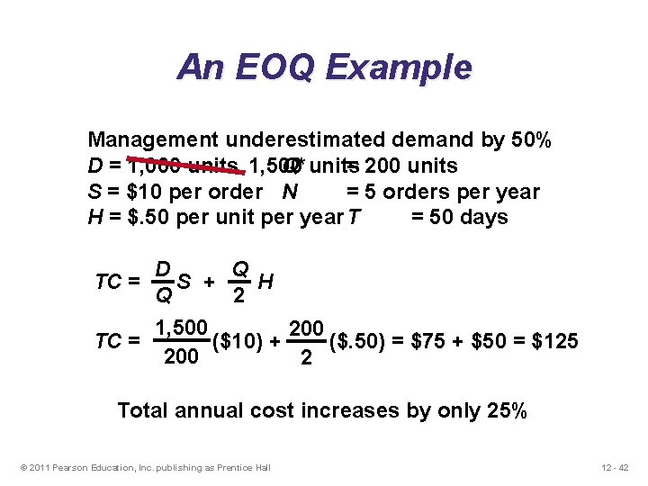
An EOQ Example Management underestimated demand by 50% D = 1, 000 units 1, 500 units Q* = 200 units S = $10 per order N = 5 orders per year H = $. 50 per unit per year. T = 50 days Q D TC = S + H 2 Q 1, 500 200 TC = ($10) + ($. 50) = $75 + $50 = $125 200 2 Total annual cost increases by only 25% © 2011 Pearson Education, Inc. publishing as Prentice Hall 12 - 42

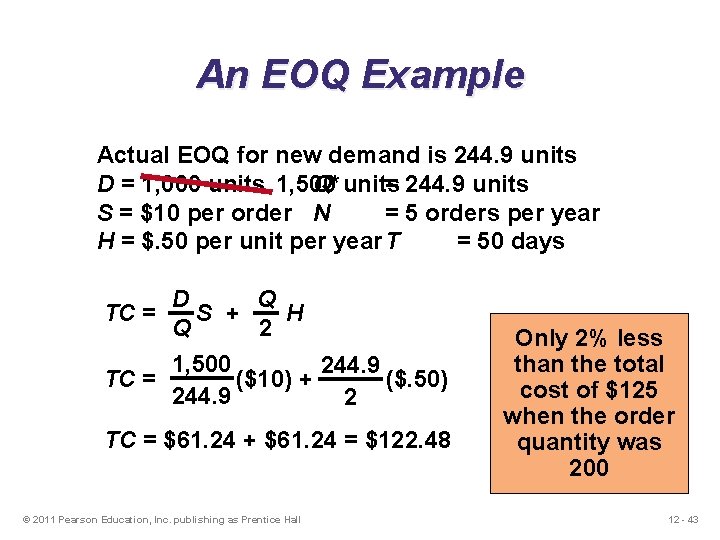
An EOQ Example Actual EOQ for new demand is 244. 9 units D = 1, 000 units 1, 500 units Q* = 244. 9 units S = $10 per order N = 5 orders per year H = $. 50 per unit per year. T = 50 days Q D TC = S + H 2 Q 1, 500 244. 9 TC = ($10) + ($. 50) 244. 9 2 TC = $61. 24 + $61. 24 = $122. 48 © 2011 Pearson Education, Inc. publishing as Prentice Hall Only 2% less than the total cost of $125 when the order quantity was 200 12 - 43

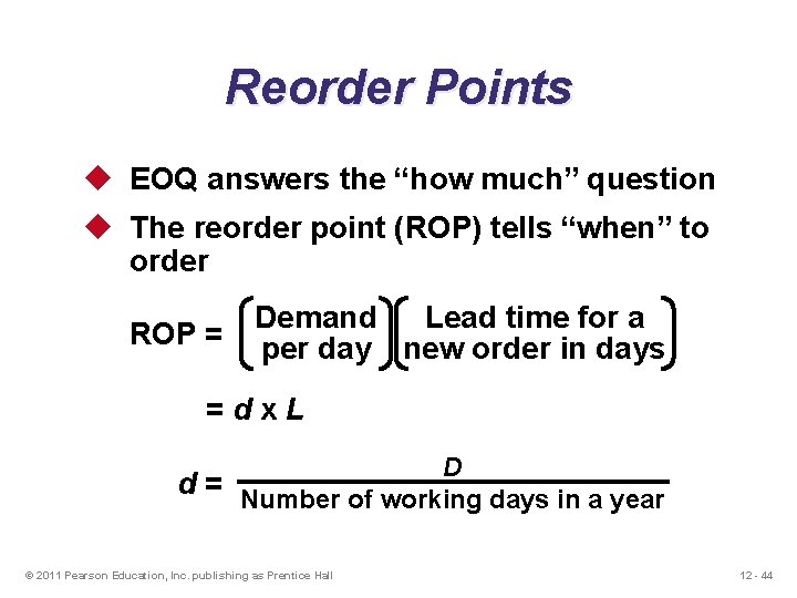
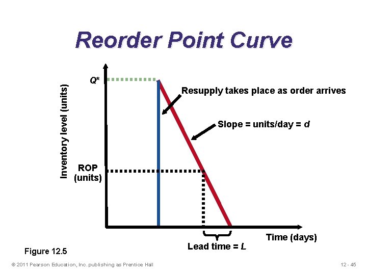
Reorder Points u EOQ answers the “how much” question u The reorder point (ROP) tells “when” to order ROP = Demand Lead time for a per day new order in days = d x L D d = Number of working days in a year © 2011 Pearson Education, Inc. publishing as Prentice Hall 12 - 44

Inventory level (units) Reorder Point Curve Q* Resupply takes place as order arrives Slope = units/day = d ROP (units) Figure 12. 5 © 2011 Pearson Education, Inc. publishing as Prentice Hall Lead time = L Time (days) 12 - 45

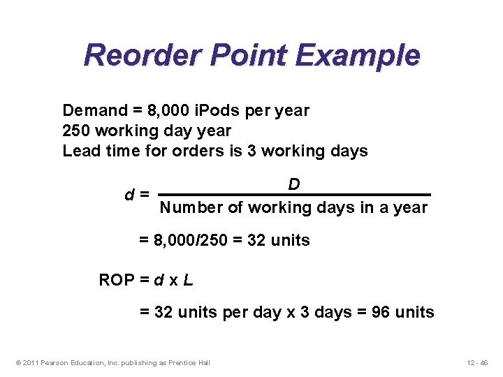
Reorder Point Example Demand = 8, 000 i. Pods per year 250 working day year Lead time for orders is 3 working days D d = Number of working days in a year = 8, 000/250 = 32 units ROP = d x L = 32 units per day x 3 days = 96 units © 2011 Pearson Education, Inc. publishing as Prentice Hall 12 - 46

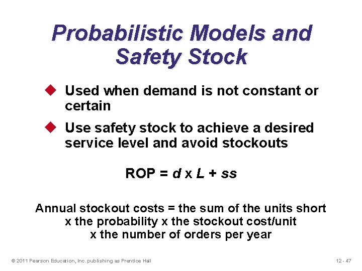
Probabilistic Models and Safety Stock u Used when demand is not constant or certain u Use safety stock to achieve a desired service level and avoid stockouts ROP = d x L + ss Annual stockout costs = the sum of the units short x the probability x the stockout cost/unit x the number of orders per year © 2011 Pearson Education, Inc. publishing as Prentice Hall 12 - 47

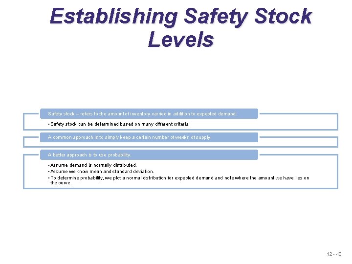
Establishing Safety Stock Levels Safety stock – refers to the amount of inventory carried in addition to expected demand. • Safety stock can be determined based on many different criteria. A common approach is to simply keep a certain number of weeks of supply. A better approach is to use probability. • Assume demand is normally distributed. • Assume we know mean and standard deviation. • To determine probability, we plot a normal distribution for expected demand note where the amount we have lies on the curve. 12 - 48

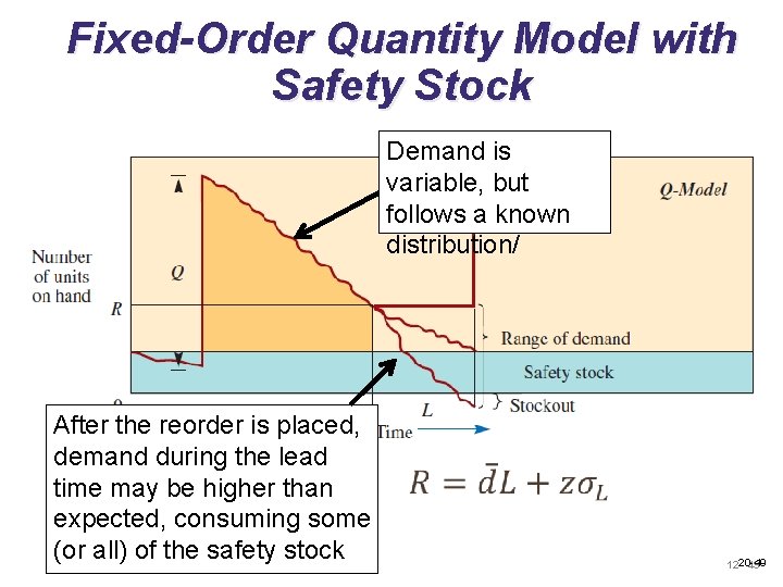
Fixed-Order Quantity Model with Safety Stock Demand is variable, but follows a known distribution/ After the reorder is placed, demand during the lead time may be higher than expected, consuming some (or all) of the safety stock 20 -49 12 - 49

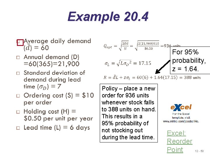
Example 20. 4 For 95% probability, z = 1. 64. Policy – place a new order for 936 units whenever stock falls to 388 units on hand. This results in a 95% probability of not stocking out during the lead time. Excel: Reorder 12 - 50 Point

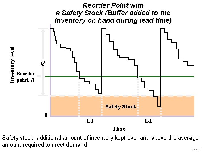
Inventory level Reorder Point with a Safety Stock (Buffer added to the inventory on hand during lead time) Q Reorder point, R Safety Stock 0 LT LT Time Safety stock: additional amount of inventory kept over and above the average amount required to meet demand 12 - 51

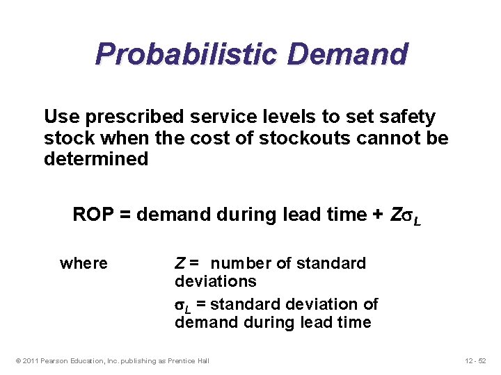
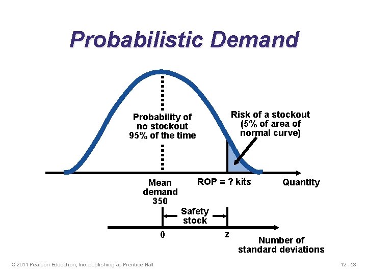
Probabilistic Demand Use prescribed service levels to set safety stock when the cost of stockouts cannot be determined ROP = demand during lead time + Zs. L where Z = number of standard deviations s. L = standard deviation of demand during lead time © 2011 Pearson Education, Inc. publishing as Prentice Hall 12 - 52

Probabilistic Demand Risk of a stockout (5% of area of normal curve) Probability of no stockout 95% of the time Mean demand 350 0 © 2011 Pearson Education, Inc. publishing as Prentice Hall ROP = ? kits Quantity Safety stock z Number of standard deviations 12 - 53

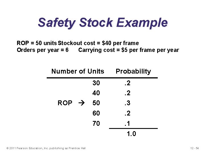
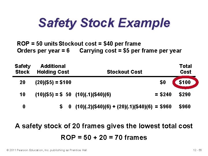
Safety Stock Example ROP = 50 units Stockout cost = $40 per frame Orders per year = 6 Carrying cost = $5 per frame per year Number of Units 30 40 ROP 50 60 70 © 2011 Pearson Education, Inc. publishing as Prentice Hall Probability. 2. 2. 3. 2. 1 1. 0 12 - 54

Safety Stock Example ROP = 50 units Stockout cost = $40 per frame Orders per year = 6 Carrying cost = $5 per frame per year Safety Additional Stock Holding Cost Stockout Cost 20 (20)($5) = $100 10 (10)($5) = $ 50 (10)(. 1)($40)(6) 0 Total Cost $0 $100 = $240 $290 $ 0 (10)(. 2)($40)(6) + (20)(. 1)($40)(6) = $960 A safety stock of 20 frames gives the lowest total cost ROP = 50 + 20 = 70 frames © 2011 Pearson Education, Inc. publishing as Prentice Hall 12 - 55

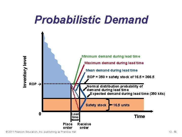
Inventory level Probabilistic Demand Minimum demand during lead time Maximum demand during lead time Mean demand during lead time ROP = 350 + safety stock of 16. 5 = 366. 5 ROP Normal distribution probability of demand during lead time Expected demand during lead time (350 kits) Safety stock 0 Lead time Place order © 2011 Pearson Education, Inc. publishing as Prentice Hall 16. 5 units Time Receive order 12 - 56

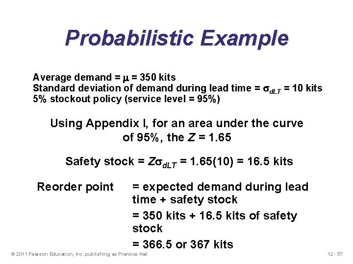
Probabilistic Example Average demand = m = 350 kits Standard deviation of demand during lead time = sd. LT = 10 kits 5% stockout policy (service level = 95%) Using Appendix I, for an area under the curve of 95%, the Z = 1. 65 Safety stock = Zsd. LT = 1. 65(10) = 16. 5 kits Reorder point = expected demand during lead time + safety stock = 350 kits + 16. 5 kits of safety stock = 366. 5 or 367 kits © 2011 Pearson Education, Inc. publishing as Prentice Hall 12 - 57

Fixed-Period (P) Systems u Orders placed at the end of a fixed period u Inventory counted only at end of period u Order brings inventory up to target level u Only relevant costs are ordering and holding u Lead times are known and constant u Items are independent from one another © 2011 Pearson Education, Inc. publishing as Prentice Hall 12 - 58

Fixed-Period Systems u Inventory is only counted at each review period u May be scheduled at convenient times u Appropriate in routine situations u May result in stockouts between periods u May require increased safety stock © 2011 Pearson Education, Inc. publishing as Prentice Hall 12 - 59

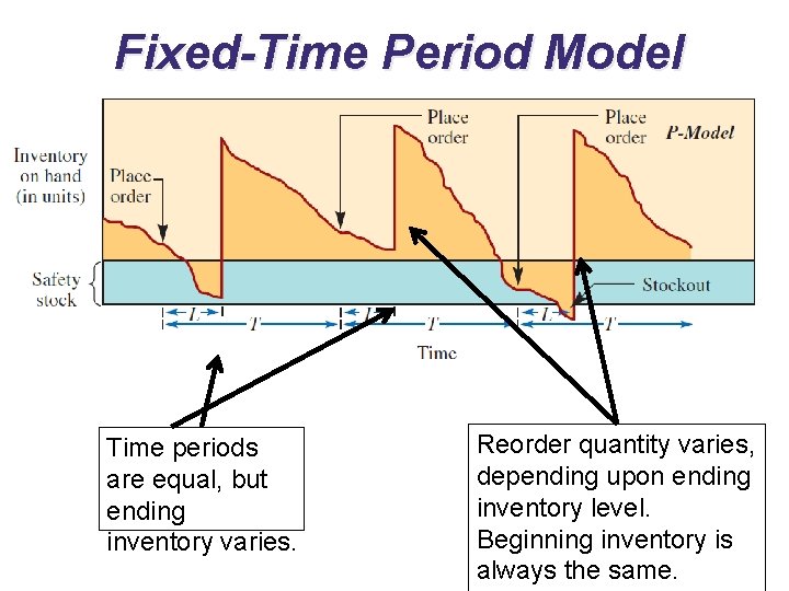
Fixed-Time Period Model Time periods are equal, but ending inventory varies. Reorder quantity varies, depending upon ending inventory level. Beginning inventory is 12 - 60 always the same.

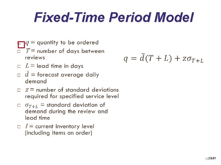
Fixed-Time Period Model 20 -61 12 - 61

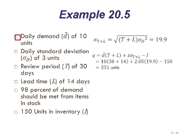
Example 20. 5 12 - 62

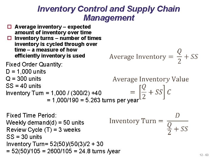
Inventory Control and Supply Chain Management Average inventory – expected amount of inventory over time Inventory turns – number of times inventory is cycled through over time – a measure of how efficiently inventory is used Fixed Order Quantity: D = 1, 000 units Q = 300 units SS = 40 units Inventory Turn = 1, 000 / (300/2) +40 = 1, 000/190 = 5. 263 turns per year Fixed Time Period: Weekly demand(d) = 50 units Review Cycle (T) = 3 weeks SS = 30 units Inventory Turn= 52(50)/(50(3)/2 + 30 = 52(50)/105 = 2600/105 = 24. 8 turns /year 12 - 63

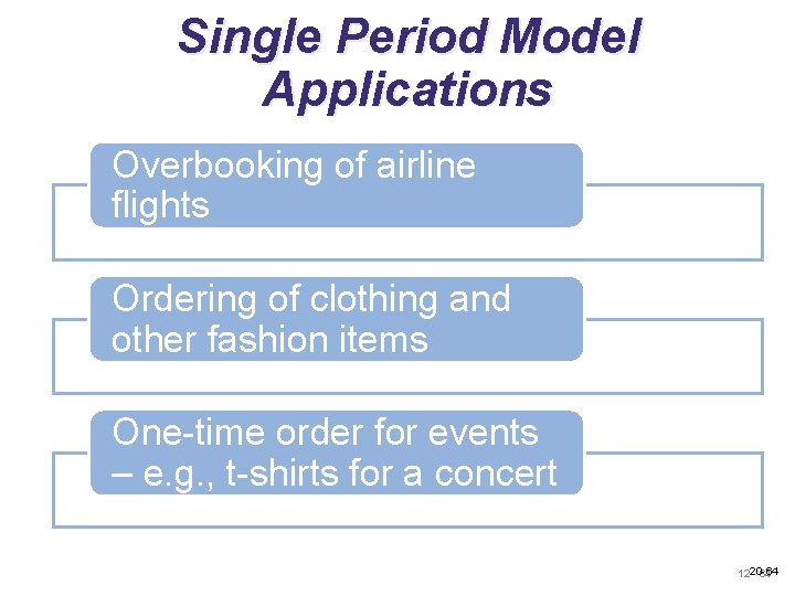
Single Period Model Applications Overbooking of airline flights Ordering of clothing and other fashion items One-time order for events – e. g. , t-shirts for a concert 20 -64 12 - 64

Single Period Inventory Model Consider the problem of deciding how many newspapers to put in a hotel lobby Too few papers and some customers will not be able to purchase a paper, and profits associated with these potential sales are lost. Too many papers and the price paid for papers that were not sold during the day will be wasted, lowering profit. 20 -65 12 - 65

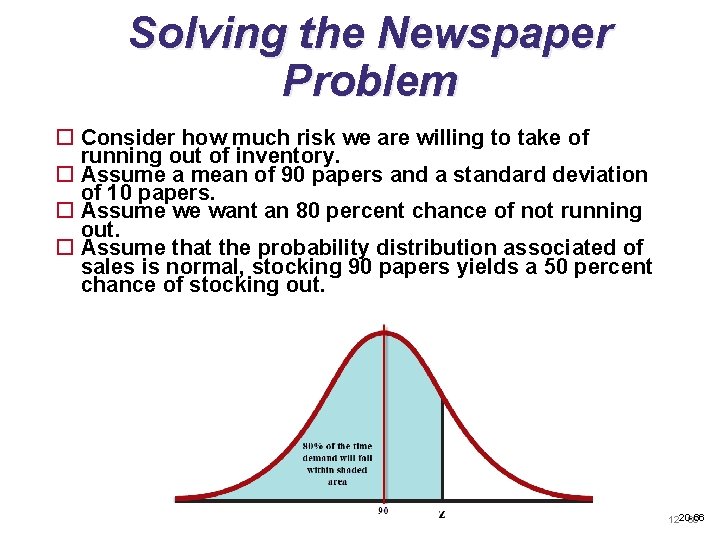
Solving the Newspaper Problem Consider how much risk we are willing to take of running out of inventory. Assume a mean of 90 papers and a standard deviation of 10 papers. Assume we want an 80 percent chance of not running out. Assume that the probability distribution associated of sales is normal, stocking 90 papers yields a 50 percent chance of stocking out. 20 -66 12 - 66

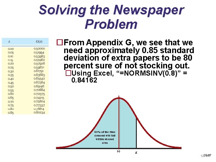
Solving the Newspaper Problem From Appendix G, we see that we need approximately 0. 85 standard deviation of extra papers to be 80 percent sure of not stocking out. �Using Excel, “=NORMSINV(0. 8)” = 0. 84162 20 -67 12 - 67

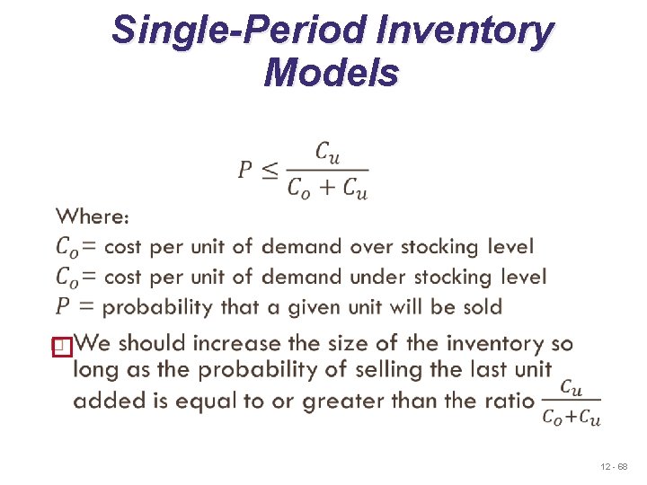
Single-Period Inventory Models 12 - 68

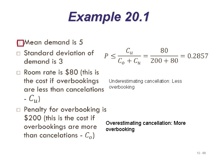
Example 20. 1 Underestimating cancellation: Less overbooking Overestimating cancellation: More overbooking 12 - 69

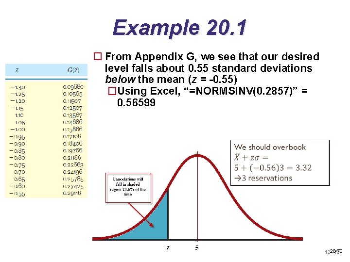
Example 20. 1 From Appendix G, we see that our desired level falls about 0. 55 standard deviations below the mean (z = -0. 55) �Using Excel, “=NORMSINV(0. 2857)” = 0. 56599 20 -70 12 - 70

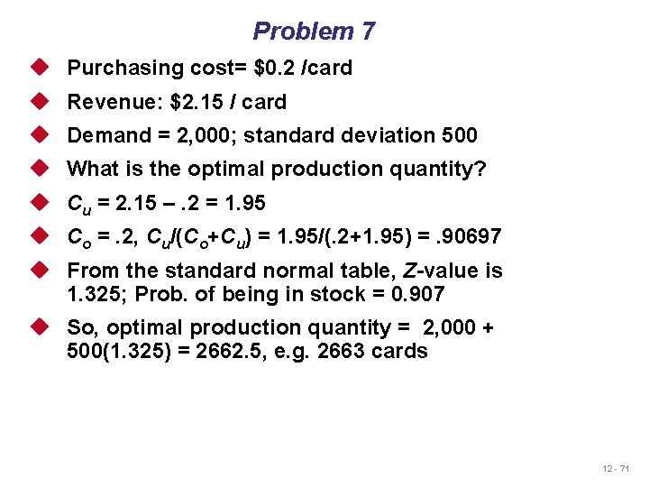
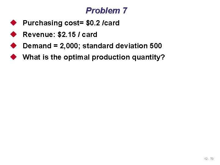
Problem 7 u Purchasing cost= $0. 2 /card u Revenue: $2. 15 / card u Demand = 2, 000; standard deviation 500 u What is the optimal production quantity? u Cu = 2. 15 –. 2 = 1. 95 u Co =. 2, Cu/(Co+Cu) = 1. 95/(. 2+1. 95) =. 90697 u From the standard normal table, Z-value is 1. 325; Prob. of being in stock = 0. 907 u So, optimal production quantity = 2, 000 + 500(1. 325) = 2662. 5, e. g. 2663 cards 12 - 71

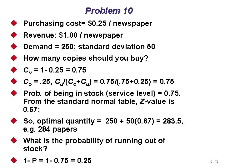
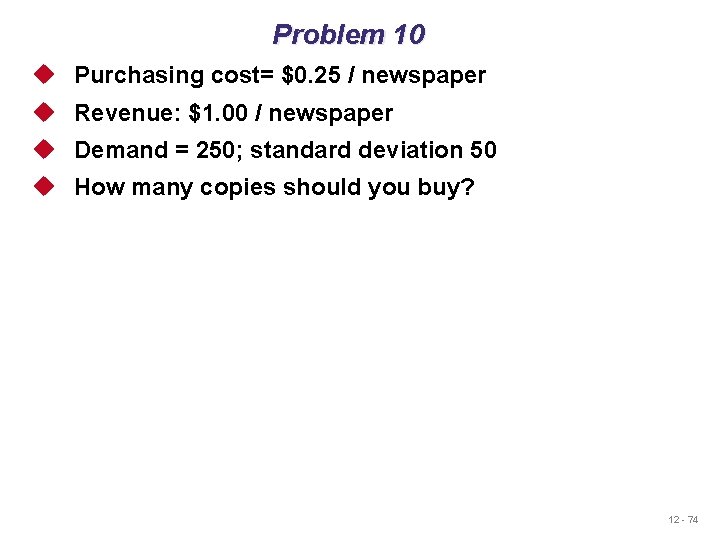
Problem 10 u Purchasing cost= $0. 25 / newspaper u Revenue: $1. 00 / newspaper u Demand = 250; standard deviation 50 u How many copies should you buy? u Cu = 1 - 0. 25 = 0. 75 u Co =. 25, Cu/(Co+Cu) = 0. 75/(. 75+0. 25) = 0. 75 u Prob. of being in stock (service level) = 0. 75. From the standard normal table, Z-value is 0. 67; u So, optimal quantity = 250 + 50(0. 67) = 283. 5, e. g. 284 papers u What is the probability of running out of stock? u 1 - P = 1 - 0. 75 = 0. 25 12 - 72

Problem 7 u Purchasing cost= $0. 2 /card u Revenue: $2. 15 / card u Demand = 2, 000; standard deviation 500 u What is the optimal production quantity? 12 - 73

Problem 10 u Purchasing cost= $0. 25 / newspaper u Revenue: $1. 00 / newspaper u Demand = 250; standard deviation 50 u How many copies should you buy? 12 - 74