Introduction to Algorithms Dynamic Programming CSE 680 Prof

Introduction to Algorithms Dynamic Programming CSE 680 Prof. Roger Crawfis

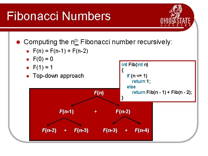
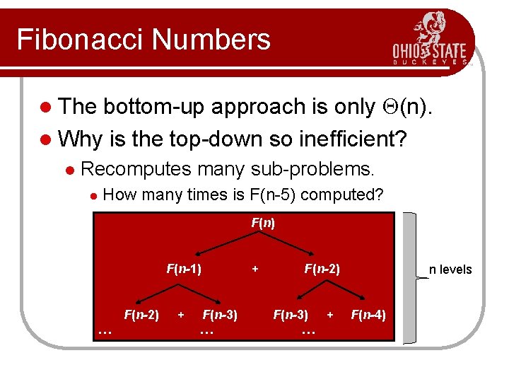
Fibonacci Numbers l Computing the nth Fibonacci number recursively: l l F(n) = F(n-1) + F(n-2) F(0) = 0 F(1) = 1 Top-down approach F(n) F(n-1) + F(n-2) + int Fib(int n) { if (n <= 1) return 1; else return Fib(n - 1) + Fib(n - 2); } F(n-2) F(n-3) + F(n-4)

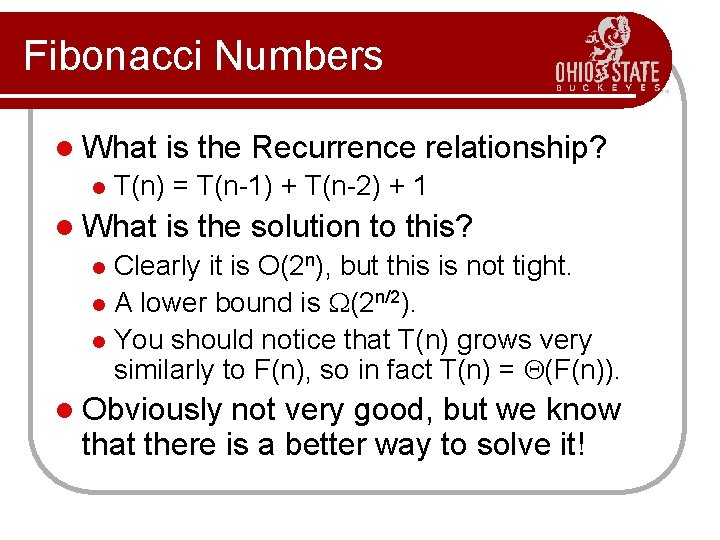
Fibonacci Numbers l What l is the Recurrence relationship? T(n) = T(n-1) + T(n-2) + 1 l What is the solution to this? Clearly it is O(2 n), but this is not tight. l A lower bound is (2 n/2). l You should notice that T(n) grows very similarly to F(n), so in fact T(n) = (F(n)). l l Obviously not very good, but we know that there is a better way to solve it!

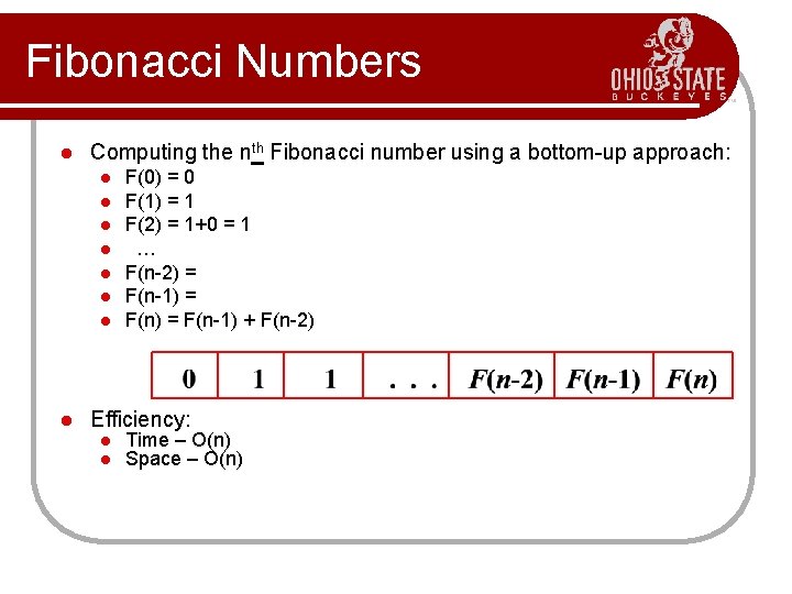
Fibonacci Numbers l Computing the nth Fibonacci number using a bottom-up approach: l l l l F(0) = 0 F(1) = 1 F(2) = 1+0 = 1 … F(n-2) = F(n-1) + F(n-2) Efficiency: l l Time – O(n) Space – O(n)

Fibonacci Numbers bottom-up approach is only (n). l Why is the top-down so inefficient? l The l Recomputes many sub-problems. l How many times is F(n-5) computed? F(n) F(n-1) + F(n-2) + … F(n-2) F(n-3) + … … n levels F(n-4)

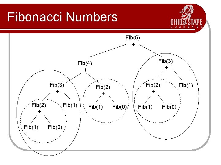
Fibonacci Numbers Fib(5) + Fib(3) + Fib(4) + Fib(3) + Fib(2) + Fib(1) Fib(0) Fib(1) Fib(0)

Dynamic Programming is an algorithm design technique for optimization problems: often minimizing or maximizing. l Like divide and conquer, DP solves problems by combining solutions to subproblems. l Unlike divide and conquer, sub-problems are not independent. l l Sub-problems may share sub-problems,

Dynamic Programming l l l The term Dynamic Programming comes from Control Theory, not computer science. Programming refers to the use of tables (arrays) to construct a solution. In dynamic programming we usually reduce time by increasing the amount of space We solve the problem by solving sub-problems of increasing size and saving each optimal solution in a table (usually). The table is then used for finding the optimal solution to larger problems. Time is saved since each sub-problem is solved only once.

Dynamic Programming l The best way to get a feel for this is through some more examples. Matrix Chaining optimization l Longest Common Subsequence l 0 -1 Knapsack Problem l Transitive Closure of a direct graph l

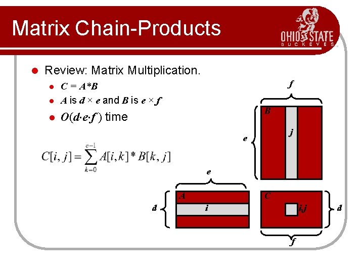
Matrix Chain-Products l Review: Matrix Multiplication. l C = A*B A is d × e and B is e × f l O(d e f ) time l f B j e e A d C i i, j f d

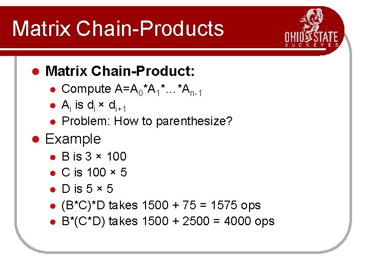
Matrix Chain-Products l Matrix Chain-Product: l l Compute A=A 0*A 1*…*An-1 Ai is di × di+1 Problem: How to parenthesize? Example l l l B is 3 × 100 C is 100 × 5 D is 5 × 5 (B*C)*D takes 1500 + 75 = 1575 ops B*(C*D) takes 1500 + 2500 = 4000 ops

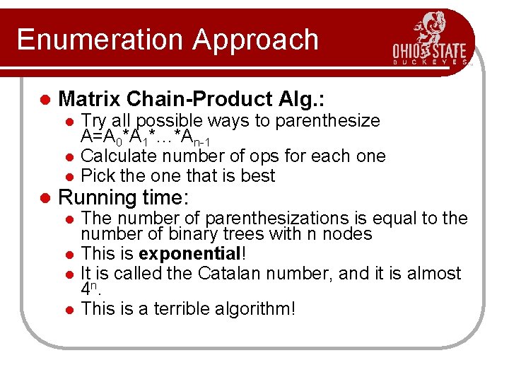
Enumeration Approach l Matrix Chain-Product Alg. : l l Try all possible ways to parenthesize A=A 0*A 1*…*An-1 Calculate number of ops for each one Pick the one that is best Running time: l l The number of parenthesizations is equal to the number of binary trees with n nodes This is exponential! It is called the Catalan number, and it is almost 4 n. This is a terrible algorithm!

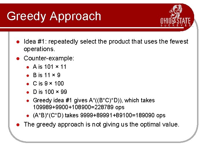
Greedy Approach Idea #1: repeatedly select the product that uses the fewest operations. l Counter-example: l l l l A is 101 × 11 B is 11 × 9 C is 9 × 100 D is 100 × 99 Greedy idea #1 gives A*((B*C)*D)), which takes 109989+9900+108900=228789 ops (A*B)*(C*D) takes 9999+89991+89100=189090 ops The greedy approach is not giving us the optimal value.

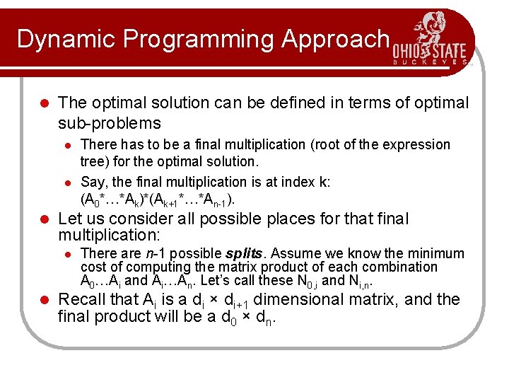
Dynamic Programming Approach l The optimal solution can be defined in terms of optimal sub-problems l l l Let us consider all possible places for that final multiplication: l l There has to be a final multiplication (root of the expression tree) for the optimal solution. Say, the final multiplication is at index k: (A 0*…*Ak)*(Ak+1*…*An-1). There are n-1 possible splits. Assume we know the minimum cost of computing the matrix product of each combination A 0…Ai and Ai…An. Let’s call these N 0, i and Ni, n. Recall that Ai is a di × di+1 dimensional matrix, and the final product will be a d 0 × dn.

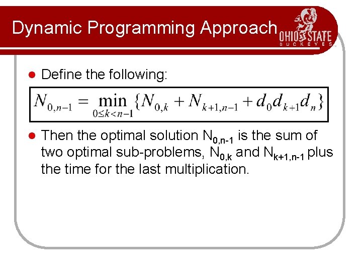
Dynamic Programming Approach l Define the following: l Then the optimal solution N 0, n-1 is the sum of two optimal sub-problems, N 0, k and Nk+1, n-1 plus the time for the last multiplication.

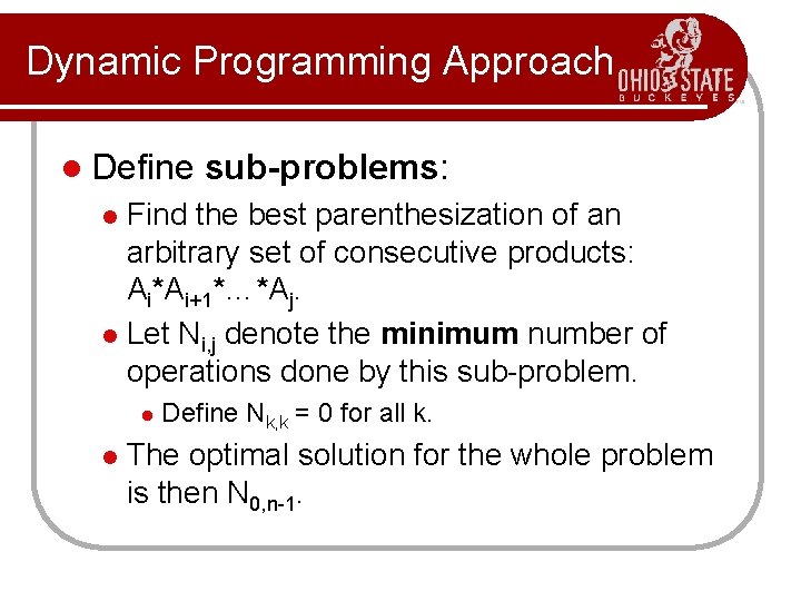
Dynamic Programming Approach l Define sub-problems: Find the best parenthesization of an arbitrary set of consecutive products: Ai*Ai+1*…*Aj. l Let Ni, j denote the minimum number of operations done by this sub-problem. l l l Define Nk, k = 0 for all k. The optimal solution for the whole problem is then N 0, n-1.

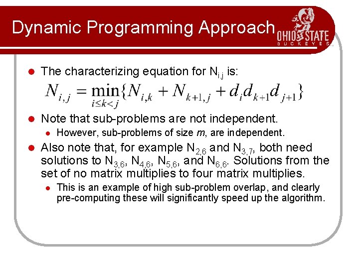
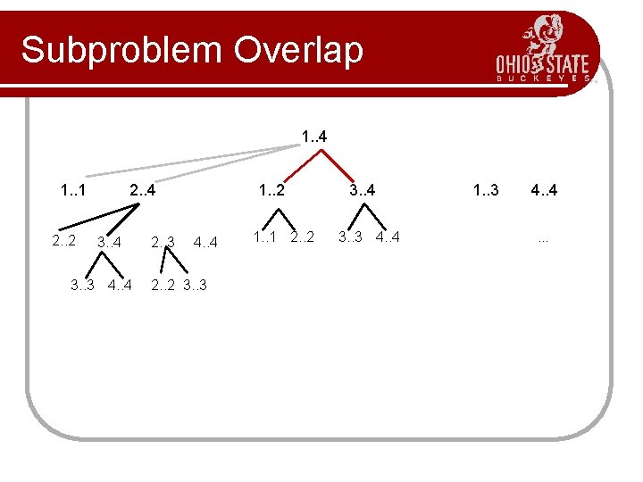
Dynamic Programming Approach l The characterizing equation for Ni, j is: l Note that sub-problems are not independent. l l However, sub-problems of size m, are independent. Also note that, for example N 2, 6 and N 3, 7, both need solutions to N 3, 6, N 4, 6, N 5, 6, and N 6, 6. Solutions from the set of no matrix multiplies to four matrix multiplies. l This is an example of high sub-problem overlap, and clearly pre-computing these will significantly speed up the algorithm.

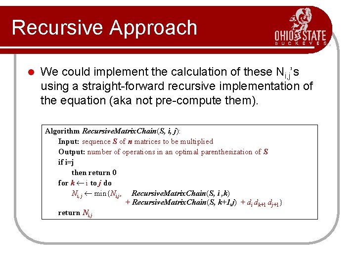
Recursive Approach l We could implement the calculation of these Ni, j’s using a straight-forward recursive implementation of the equation (aka not pre-compute them). Algorithm Recursive. Matrix. Chain(S, i, j): Input: sequence S of n matrices to be multiplied Output: number of operations in an optimal parenthesization of S if i=j then return 0 for k i to j do Ni, j min{Ni, j, Recursive. Matrix. Chain(S, i , k) + Recursive. Matrix. Chain(S, k+1, j) + di dk+1 dj+1} return Ni, j

Subproblem Overlap 1. . 4 1. . 1 2. . 2 2. . 4 3. . 3 4. . 4 2. . 3 1. . 2 4. . 4 2. . 2 3. . 3 1. . 1 2. . 2 3. . 4 3. . 3 4. . 4 1. . 3 4. . .

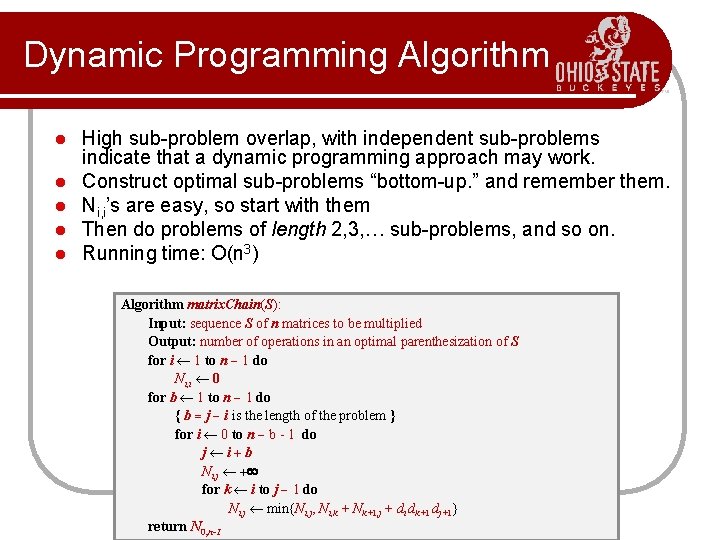
Dynamic Programming Algorithm l l l High sub-problem overlap, with independent sub-problems indicate that a dynamic programming approach may work. Construct optimal sub-problems “bottom-up. ” and remember them. Ni, i’s are easy, so start with them Then do problems of length 2, 3, … sub-problems, and so on. Running time: O(n 3) Algorithm matrix. Chain(S): Input: sequence S of n matrices to be multiplied Output: number of operations in an optimal parenthesization of S for i 1 to n - 1 do Ni, i 0 for b 1 to n - 1 do { b = j - i is the length of the problem } for i 0 to n - b - 1 do j i+b Ni, j + for k i to j - 1 do Ni, j min{Ni, j, Ni, k + Nk+1, j + di dk+1 dj+1} return N 0, n-1

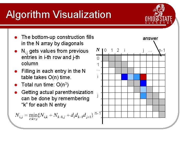
Algorithm Visualization l l l The bottom-up construction fills in the N array by diagonals Ni, j gets values from previous N entries in i-th row and j-th 0 column 1 … Filling in each entry in the N i table takes O(n) time. Total run time: O(n 3) Getting actual parenthesization j can be done by remembering “k” for each N entry n-1 answer 0 1 2 i j … n-1

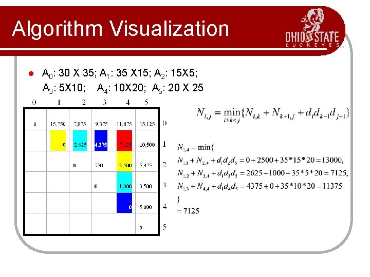
Algorithm Visualization l A 0: 30 X 35; A 1: 35 X 15; A 2: 15 X 5; A 3: 5 X 10; A 4: 10 X 20; A 5: 20 X 25

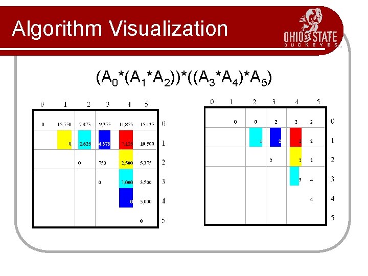
Algorithm Visualization (A 0*(A 1*A 2))*((A 3*A 4)*A 5)

Matrix Chain-Products l Some final thoughts We reduced replaced a O(2 n) algorithm with a (n 3) algorithm. l While the generic top-down recursive algorithm would have solved O(2 n) subproblems, there are (n 2) sub-problems. l l l Implies a high overlap of sub-problems. The sub-problems are independent: l Solution to A 0 A 1…Ak is independent of the solution to Ak+1…An.

Matrix Chain-Products Summary l Determine the cost of each pair-wise multiplication, then the minimum cost of multiplying three consecutive matrices (2 possible choices), using the precomputed costs for two matrices. l Repeat until we compute the minimum cost of all n matrices using the costs of the minimum n-1 matrix product costs. l n-1 possible choices.