CSE 202 Algorithms Dynamic Programming 5103 CSE 202
![LCS has “optimal substructure” Suppose length(X) = x and length(Y)=y. Let X[a: b] mean LCS has “optimal substructure” Suppose length(X) = x and length(Y)=y. Let X[a: b] mean](https://slidetodoc.com/presentation_image_h/8ff437dc25bd8efe7d6ab95b85fda4aa/image-7.jpg)
![Dynamic Programming for LCS Table: L(i, j) = length of LCS ( X[1: i], Dynamic Programming for LCS Table: L(i, j) = length of LCS ( X[1: i],](https://slidetodoc.com/presentation_image_h/8ff437dc25bd8efe7d6ab95b85fda4aa/image-8.jpg)
- Slides: 22

CSE 202 - Algorithms • Dynamic Programming 5/1/03 CSE 202 - Dynamic Programming

Chess Endgames • Ken Thompson (Bell Labs) solved all chess endgame positions with 5 pieces (1986). Some surprises: – K+Q beats K+2 B. (Since 1634, believed to be draw). – 50 moves without a pawn move or capture is not sufficient to ensure it’s a draw. – By now, most (all? ) 6 -piece endgames are solved too. • Searching all possible games with 5 pieces, going forward 50 or so moves, is infeasible (today). – If typical position has 4 moves, search is 2100 long – 2100 = 245 ops/second x 225 seconds/year x 1 billion years. • There is a better way! 2 CSE 202 - Dynamic Programming

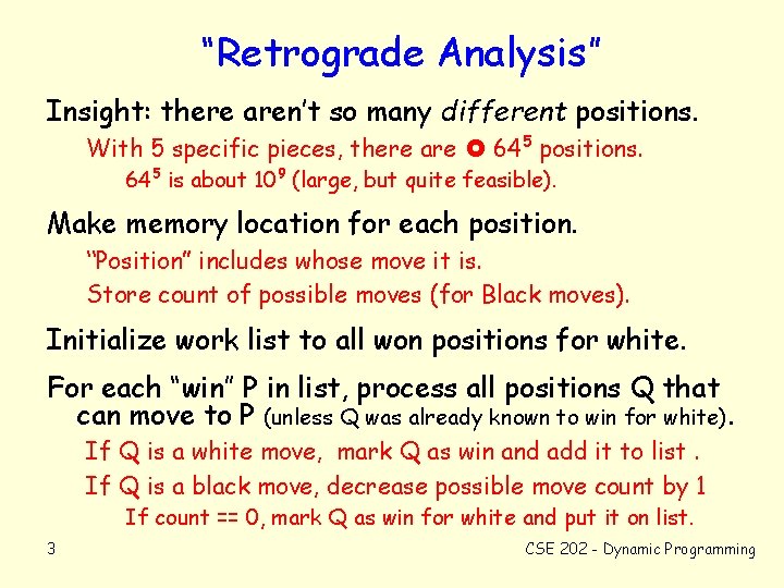
“Retrograde Analysis” Insight: there aren’t so many different positions. With 5 specific pieces, there are 645 positions. 645 is about 109 (large, but quite feasible). Make memory location for each position. “Position” includes whose move it is. Store count of possible moves (for Black moves). Initialize work list to all won positions for white. For each “win” P in list, process all positions Q that can move to P (unless Q was already known to win for white). If Q is a white move, mark Q as win and add it to list. If Q is a black move, decrease possible move count by 1 If count == 0, mark Q as win for white and put it on list. 3 CSE 202 - Dynamic Programming

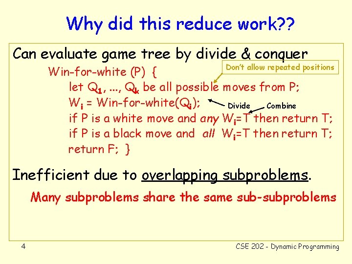
Why did this reduce work? ? Can evaluate game tree by divide & conquer Don’t allow repeated positions Win-for-white (P) { let Q 1, . . . , Qk be all possible moves from P; Wi = Win-for-white(Qi); Divide Combine if P is a white move and any Wi=T then return T; if P is a black move and all Wi=T then return T; return F; } Inefficient due to overlapping subproblems. Many subproblems share the same sub-subproblems 4 CSE 202 - Dynamic Programming

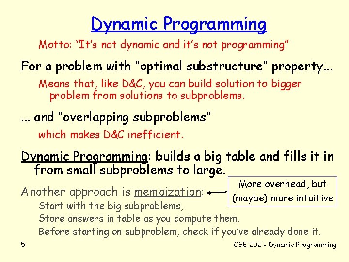
Dynamic Programming Motto: “It’s not dynamic and it’s not programming” For a problem with “optimal substructure” property. . . Means that, like D&C, you can build solution to bigger problem from solutions to subproblems. . and “overlapping subproblems” which makes D&C inefficient. Dynamic Programming: builds a big table and fills it in from small subproblems to large. Another approach is memoization: More overhead, but (maybe) more intuitive 5 CSE 202 - Dynamic Programming Start with the big subproblems, Store answers in table as you compute them. Before starting on subproblem, check if you’ve already done it.

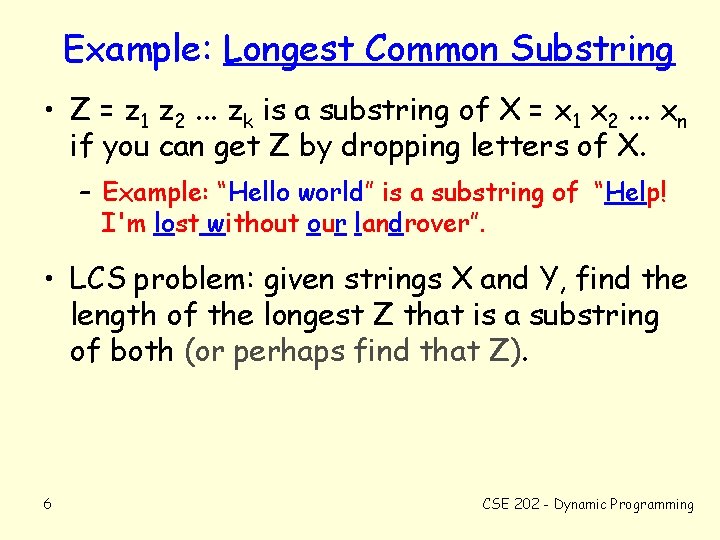
Example: Longest Common Substring • Z = z 1 z 2. . . zk is a substring of X = x 1 x 2. . . xn if you can get Z by dropping letters of X. – Example: “Hello world” is a substring of “Help! I'm lost without our landrover”. • LCS problem: given strings X and Y, find the length of the longest Z that is a substring of both (or perhaps find that Z). 6 CSE 202 - Dynamic Programming
![LCS has optimal substructure Suppose lengthX x and lengthYy Let Xa b mean LCS has “optimal substructure” Suppose length(X) = x and length(Y)=y. Let X[a: b] mean](https://slidetodoc.com/presentation_image_h/8ff437dc25bd8efe7d6ab95b85fda4aa/image-7.jpg)
LCS has “optimal substructure” Suppose length(X) = x and length(Y)=y. Let X[a: b] mean the a-th to b-th character of X. Observation: If Z is a substring of X and Y, then the last character of Z is the last character of both X and Y. . . so LCS(X, Y) = LCS( X[1: x-1], Y[1: y-1] ) || X[x] or of just X, so LCS(X, Y) = LCS(X, Y[1: y-1]) or of just Y, so LCS(X, Y) = LCS(X[1: x-1], Y) or neither so LCS(X, Y) = LCS(X[1: x-1], Y[1: y-1]) 7 CSE 202 - Dynamic Programming
![Dynamic Programming for LCS Table Li j length of LCS X1 i Dynamic Programming for LCS Table: L(i, j) = length of LCS ( X[1: i],](https://slidetodoc.com/presentation_image_h/8ff437dc25bd8efe7d6ab95b85fda4aa/image-8.jpg)
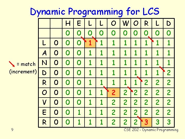
Dynamic Programming for LCS Table: L(i, j) = length of LCS ( X[1: i], Y[1, j] ). If the last character of both X and Y is the same. . . LCS(X, Y) = LCS(X[1: x-1], Y[1: y-1] ) || X[x] otherwise, LCS(X, Y) = LCS(X, Y[1: y-1]) or LCS(X, Y) = LCS(X[1: x-1], Y[1: y-1]) tells us: L(i, j) = max { L(i-1, j-1)+ (X[i]==Y[i]), L(i, j-1), L(i-1, j) } Each table entry is computed from 3 earlier entries. 8 CSE 202 - Dynamic Programming

Dynamic Programming for LCS = match (increment) 9 L A N D R O V E R 0 0 0 0 0 H 0 0 0 0 0 E 0 0 0 0 1 1 L 0 1 1 1 1 1 O W O R 0 0 1 1 1 1 1 2 2 2 2 3 L 0 1 1 2 2 3 D 0 1 1 1 2 2 2 3 CSE 202 - Dynamic Programming

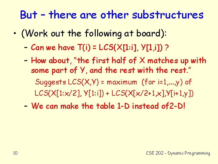
But – there are other substructures • (Work out the following at board): – Can we have T(i) = LCS(X[1: i], Y[1, i]) ? – How about, “the first half of X matches up with some part of Y, and the rest with the rest. ” Suggests LCS(X, Y) = maximum (for i=1, . . . , y) of LCS(X[1: x/2], Y[1: i]) + LCS(X[x/2+1, x], Y[i+1, y]) – We can make the table 1 -D instead of 2 -D! 10 CSE 202 - Dynamic Programming

Summary For a good dynamic programming algorithm: – Table should be low-dimensional • keeps memory requirements low. – Each table entry should be fast to calculate • keeps complexity low. May decompose problems differently than a good Divide & Conquer algorithm. 11 CSE 202 - Dynamic Programming

How to get your name on an algorithm: Use Dynamic Programming • Earley’s algorithm: Parse a string using a CFG. • Viterbi’s algorithm: Break string into codewords • Smith-Waterman algorithm: Match up two strings of DNA or protein • Floyd-Warshall: All-pairs shortest paths. 12 CSE 202 - Dynamic Programming

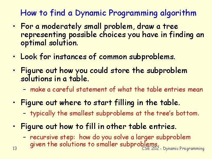
How to find a Dynamic Programming algorithm • For a moderately small problem, draw a tree representing possible choices you have in finding an optimal solution. • Look for instances of common subproblems. • Figure out how you could store the subproblem solutions in a table. – make a careful statement of what the table entries mean • Figure out where to start filling in the table. – typically the smallest subproblems at the tree’s bottom. • Figure out how to fill in other table entries. 13 – recursive step: how do you solve a larger subproblem given the solutions to smaller subproblems. CSE 202 - Dynamic Programming

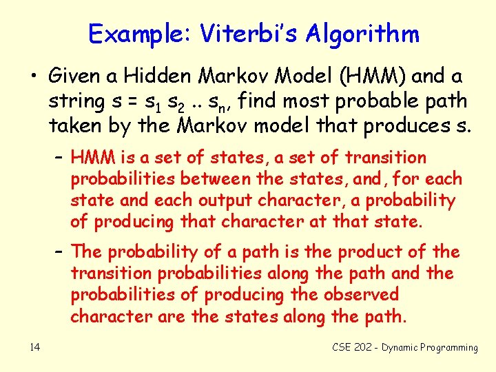
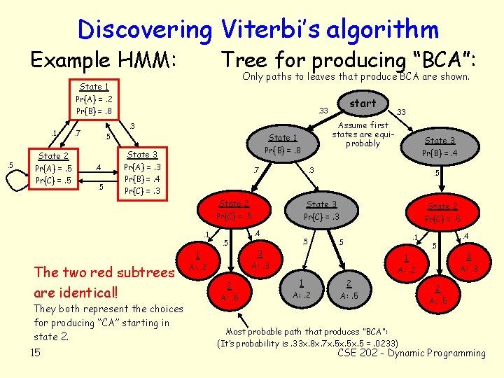
Example: Viterbi’s Algorithm • Given a Hidden Markov Model (HMM) and a string s = s 1 s 2. . sn, find most probable path taken by the Markov model that produces s. – HMM is a set of states, a set of transition probabilities between the states, and, for each state and each output character, a probability of producing that character at that state. – The probability of a path is the product of the transition probabilities along the path and the probabilities of producing the observed character are the states along the path. 14 CSE 202 - Dynamic Programming

Discovering Viterbi’s algorithm Example HMM: Tree for producing “BCA”: Only paths to leaves that produce BCA are shown. State 1 Pr{A} =. 2 Pr{B} =. 8. 1 . 5 State 2 Pr{A} =. 5 Pr{C} =. 5 State 1 Pr{B} =. 8 . 5 . 4. 5 State 3 Pr{A} =. 3 Pr{B} =. 4 Pr{C} =. 3 . 7 State 2 Pr{C} =. 5. 1 The two red subtrees are identical! They both represent the choices for producing “CA” starting in state 2. 15 1 A: . 2 2 A: . 5 State 3 Pr{B} =. 4 . 3 . 5 State 3 Pr{C} =. 3. 4 . 5 . 33 Assume first states are equiprobably . 3 . 7 start . 33 . 5 State 2 Pr{C} =. 5. 1 . 5 3 A: . 3 . 4. 5 1 A: . 2 2 A: . 5 Most probable path that produces “BCA”: (It’s probability is. 33 x. 8 x. 7 x. 5 x. 5 =. 0233) 3 A: . 3 2 A: . 5 CSE 202 - Dynamic Programming

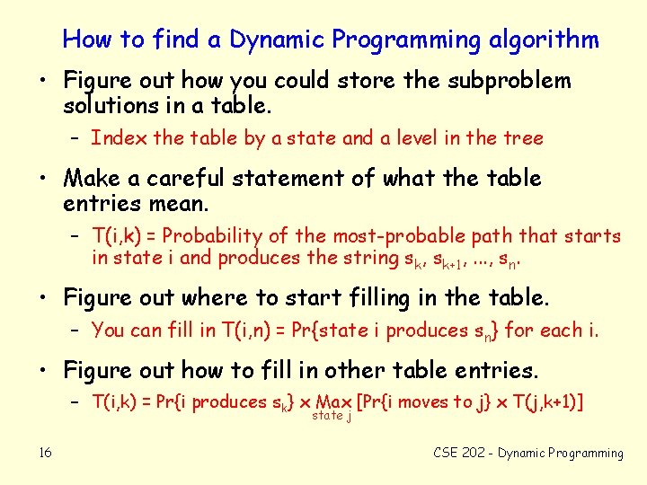
How to find a Dynamic Programming algorithm • Figure out how you could store the subproblem solutions in a table. – Index the table by a state and a level in the tree • Make a careful statement of what the table entries mean. – T(i, k) = Probability of the most-probable path that starts in state i and produces the string sk, sk+1, . . . , sn. • Figure out where to start filling in the table. – You can fill in T(i, n) = Pr{state i produces sn} for each i. • Figure out how to fill in other table entries. – T(i, k) = Pr{i produces sk} x Max [Pr{i moves to j} x T(j, k+1)] state j 16 CSE 202 - Dynamic Programming

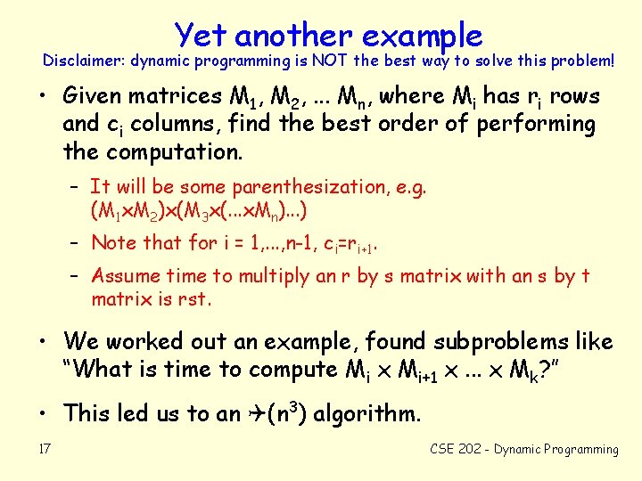
Yet another example Disclaimer: dynamic programming is NOT the best way to solve this problem! • Given matrices M 1, M 2, . . . Mn, where Mi has ri rows and ci columns, find the best order of performing the computation. – It will be some parenthesization, e. g. (M 1 x. M 2)x(M 3 x(. . . x. Mn). . . ) – Note that for i = 1, . . . , n-1, ci=ri+1. – Assume time to multiply an r by s matrix with an s by t matrix is rst. • We worked out an example, found subproblems like “What is time to compute Mi x Mi+1 x. . . x Mk? ” • This led us to an (n 3) algorithm. 17 CSE 202 - Dynamic Programming

Protein (or DNA) String Matching Biological sequences: A proteins is a string of amino acids (20 “characters”). DNA is a string of base pairs (4 “characters”). Databases of known sequences: SDSC handles the Protein Data Base (PDB). Human Genome (3 x 10⁹ base pairs) computed in ‘ 01. String matching problem: Given a query string, find similar strings in database. Smith-Waterman algorithm is most accurate method. Fast. A and BLAST are faster approximations. 18 CSE 202 - Dynamic Programming

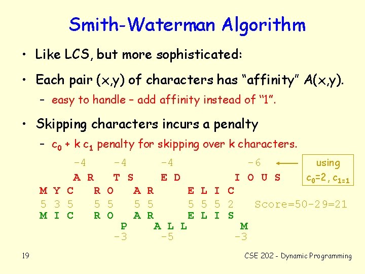
Smith-Waterman Algorithm • Like LCS, but more sophisticated: • Each pair (x, y) of characters has “affinity” A(x, y). – easy to handle – add affinity instead of “ 1”. • Skipping characters incurs a penalty – c 0 + k c 1 penalty for skipping over k characters. -4 -4 -6 using T S E D I O U S c 0=2, c 1=1 R O A R E L I C 5 5 5 5 2 Score=50 -29=21 R O A R E L I S P A L L M -3 -5 -3 -4 A R M Y C 5 3 5 M I C 19 CSE 202 - Dynamic Programming

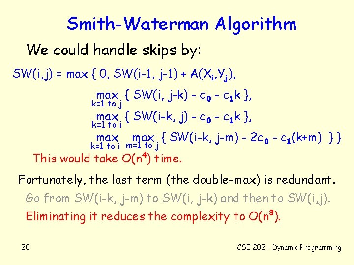
Smith-Waterman Algorithm We could handle skips by: SW(i, j) = max { 0, SW(i-1, j-1) + A(Xi, Yj), max { SW(i, j-k) - c 0 - c 1 k }, k=1 to j max { SW(i-k, j) - c 0 - c 1 k }, k=1 to i max { SW(i-k, j-m) - 2 c 0 - c 1(k+m) } } k=1 to i m=1 to j This would take O(n 4) time. Fortunately, the last term (the double-max) is redundant. Go from SW(i-k, j-m) to SW(i, j-k) and then to SW(i, j). Eliminating it reduces the complexity to O(n 3). 20 CSE 202 - Dynamic Programming

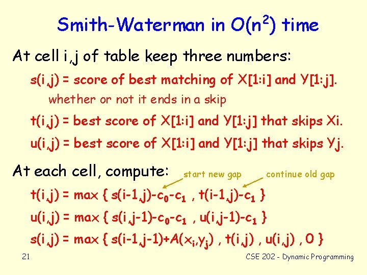
2 Smith-Waterman in O(n ) time At cell i, j of table keep three numbers: s(i, j) = score of best matching of X[1: i] and Y[1: j]. whether or not it ends in a skip t(i, j) = best score of X[1: i] and Y[1: j] that skips Xi. u(i, j) = best score of X[1: i] and Y[1: j] that skips Yj. At each cell, compute: start new gap continue old gap t(i, j) = max { s(i-1, j)-c 0 -c 1 , t(i-1, j)-c 1 } u(i, j) = max { s(i, j-1)-c 0 -c 1 , u(i, j-1)-c 1 } s(i, j) = max { s(i-1, j-1)+A(xi, yj) , t(i, j) , u(i, j) , 0 } 21 CSE 202 - Dynamic Programming

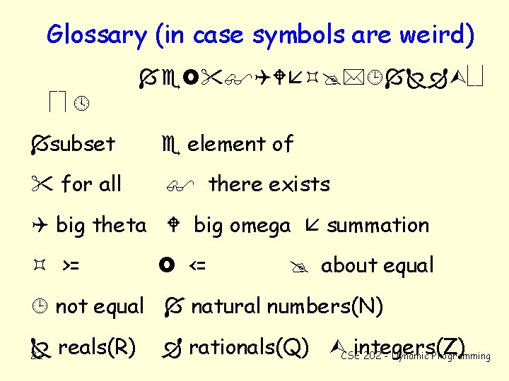
Glossary (in case symbols are weird) subset for all element of there exists big theta big omega summation >= <= about equal not equal natural numbers(N) reals(R) 22 rationals(Q) CSEintegers(Z) 202 - Dynamic Programming