Introduction to Algorithms Spanning Trees CSE 680 Prof

Introduction to Algorithms Spanning Trees CSE 680 Prof. Roger Crawfis http: //web. cse. ohio-state. edu/~crawfis. 3/cse 680/Slides/CSE 680 -15 Spanning. Trees. pptx

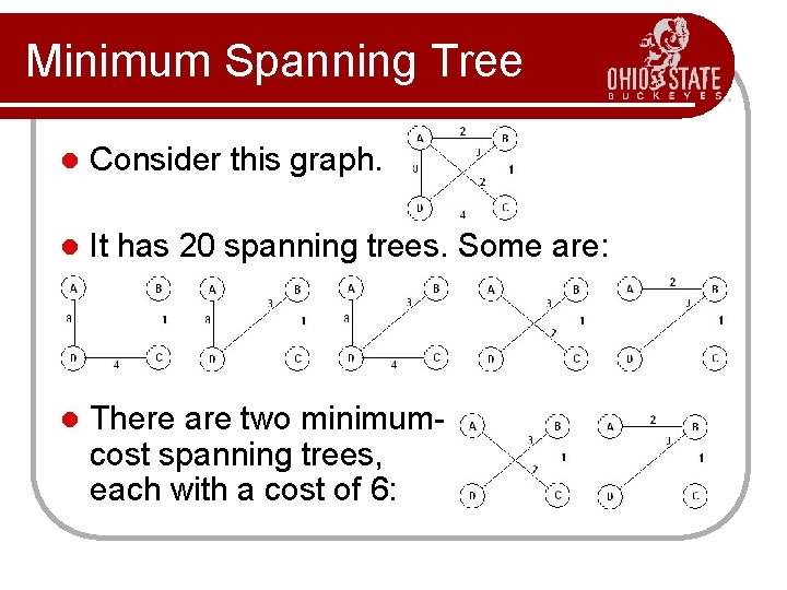
Minimum Spanning Tree l Consider this graph. l It has 20 spanning trees. Some are: l There are two minimumcost spanning trees, each with a cost of 6:

Minimum Spanning Tree There are many approaches to computing a minimum spanning tree. We could try to detect cycles and remove edges, but the two algorithms we will study build them from the bottom-up in a greedy fashion. l Kruskal’s Algorithm – starts with a forest of single node trees and then adds the edge with the minimum weight to connect two components. l Prim’s Algorithm – starts with a single vertex and then adds the minimum edge to extend the spanning tree. l

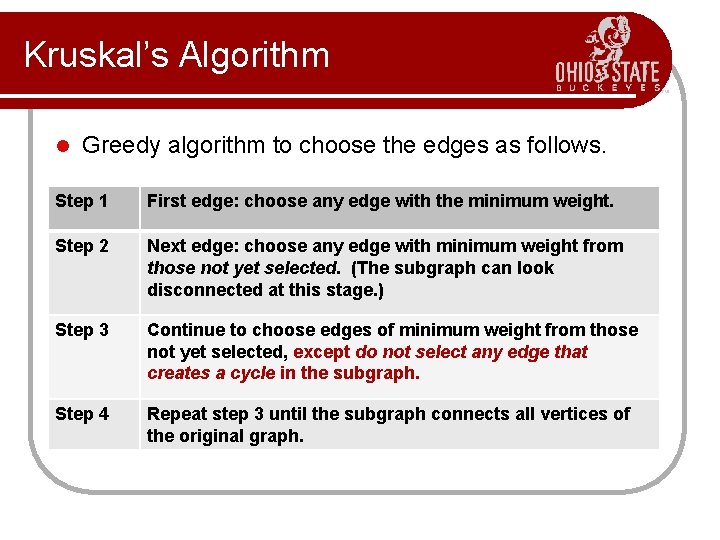
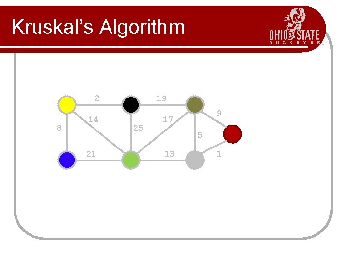
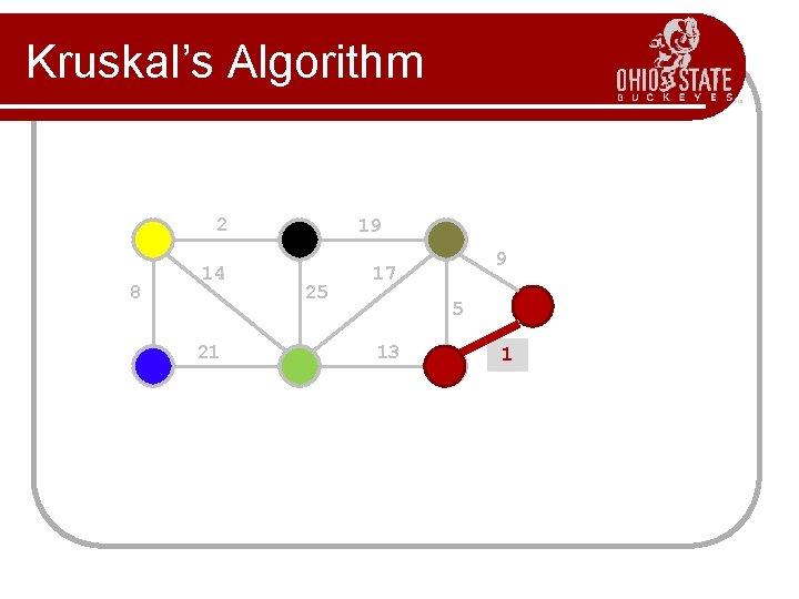
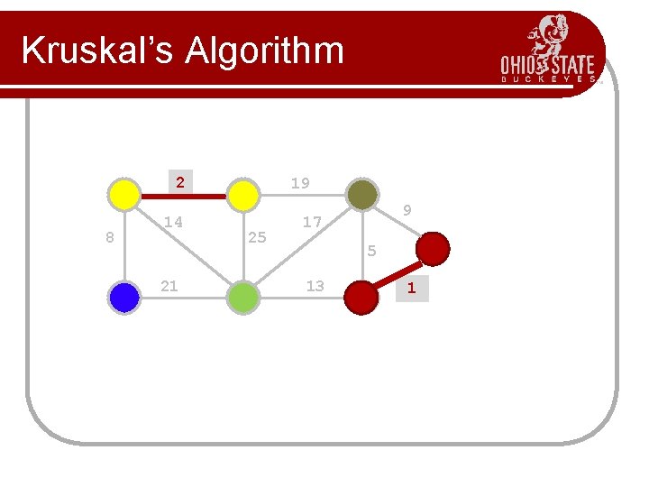
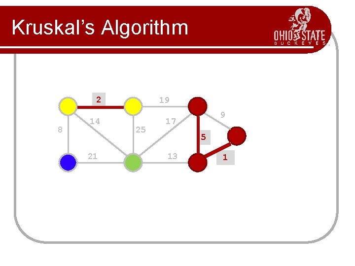
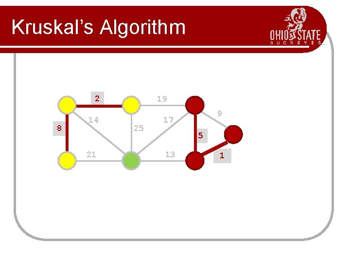
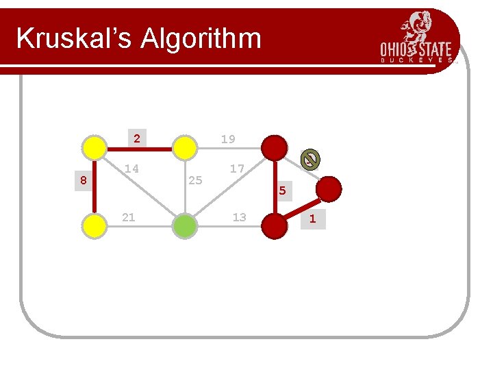
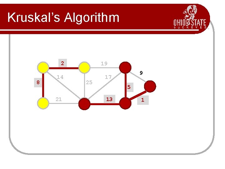
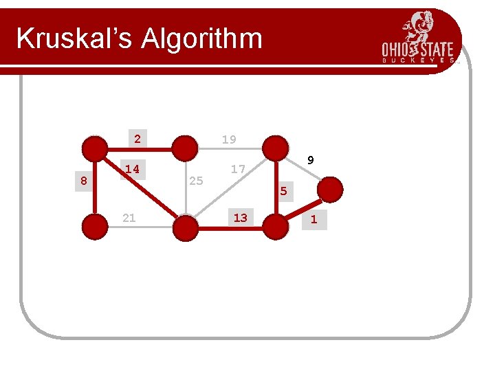
Kruskal’s Algorithm l Greedy algorithm to choose the edges as follows. Step 1 First edge: choose any edge with the minimum weight. Step 2 Next edge: choose any edge with minimum weight from those not yet selected. (The subgraph can look disconnected at this stage. ) Step 3 Continue to choose edges of minimum weight from those not yet selected, except do not select any edge that creates a cycle in the subgraph. Step 4 Repeat step 3 until the subgraph connects all vertices of the original graph.

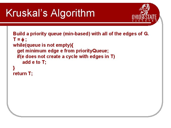
Kruskal’s Algorithm Build a priority queue (min-based) with all of the edges of G. T= ; while(queue is not empty){ get minimum edge e from priority. Queue; if(e does not create a cycle with edges in T) add e to T; } return T;

Kruskal’s Algorithm 2 8 14 21 19 25 9 17 5 13 1

Kruskal’s Algorithm 2 8 14 21 19 25 9 17 5 13 1? 1

Kruskal’s Algorithm 2 8 14 21 19 25 9 17 5 13 1? 1

Kruskal’s Algorithm 2 8 14 21 19 25 9 17 5 13 1? 1

Kruskal’s Algorithm 2 8 14 21 19 25 9 17 5 13 1? 1

Kruskal’s Algorithm 2 8 14 21 19 25 9 17 5 13 1? 1

Kruskal’s Algorithm 2 8 14 21 19 25 9 17 5 13 1? 1

Kruskal’s Algorithm 2 8 14 21 19 25 9 17 5 13 1? 1

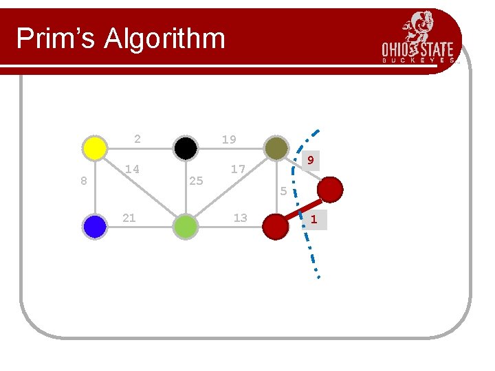
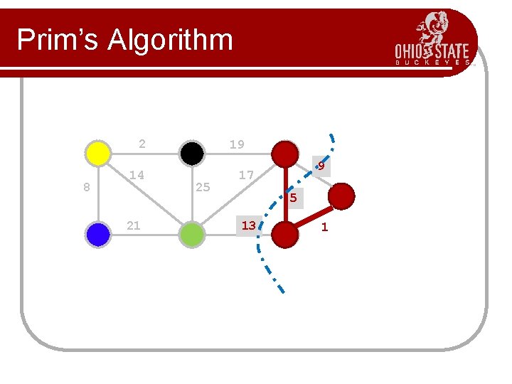
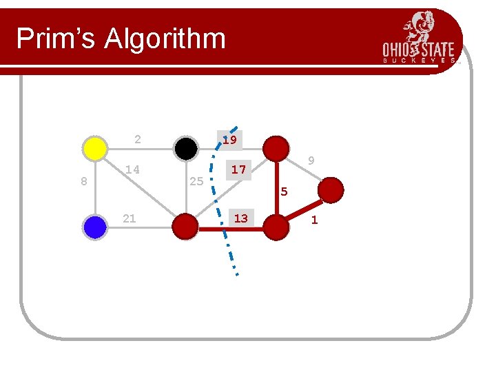
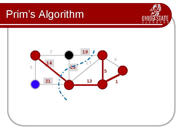
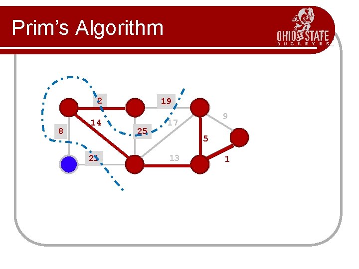
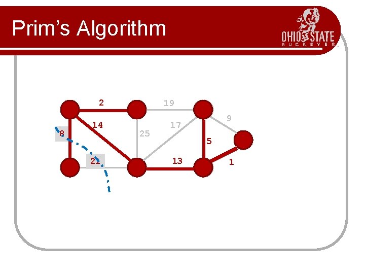
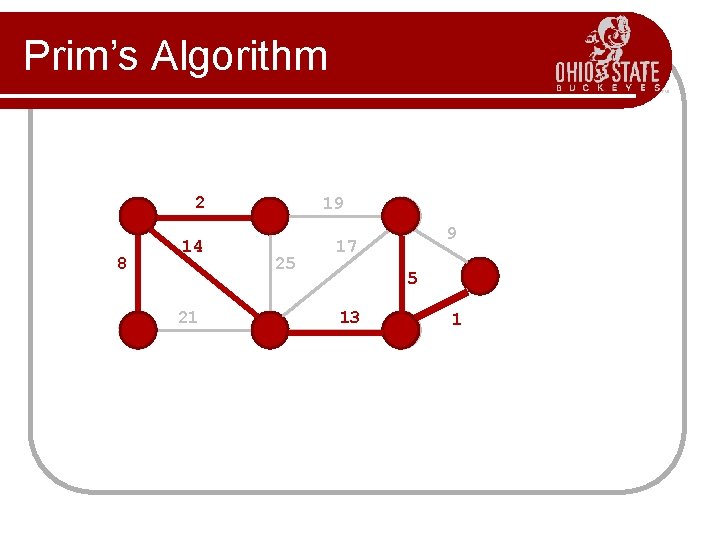
Prim’s Algorithm l l l Prim’s algorithm finds a minimum cost spanning tree by selecting edges from the graph one-by-one as follows: It starts with a tree, T, consisting of a single starting vertex, x. Then, it finds the shortest edge emanating from x that connects T to the rest of the graph (i. e. , a vertex not in the tree T). It adds this edge and the new vertex to the tree T. It then picks the shortest edge emanating from the revised tree T that also connects T to the rest of the graph and repeats the process.

Prim’s Algorithm Abstract Consider a graph G=(V, E); Let T be a tree consisting of only the starting vertex x; while (T has fewer than I V I vertices) { find a smallest edge connecting T to G-T; add it to T; }

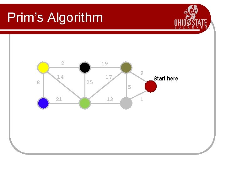
Prim’s Algorithm 2 8 14 21 19 25 9 17 5 13 1 Start here

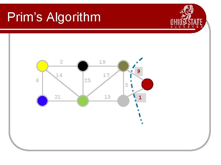
Prim’s Algorithm 2 8 14 21 19 25 9 17 5 13 1? 1

Prim’s Algorithm 2 8 14 21 19 25 9 17 5 13 1? 1

Prim’s Algorithm 2 8 14 21 19 25 9 17 5 13 1

Prim’s Algorithm 2 8 14 21 19 25 9 17 5 13 1

Prim’s Algorithm 2 8 14 21 19 25 9 17 5 13 1

Prim’s Algorithm 2 8 14 21 19 25 9 17 5 13 1

Prim’s Algorithm 2 8 14 21 19 25 9 17 5 13 1

Prim’s Algorithm 2 8 14 21 19 25 9 17 5 13 1

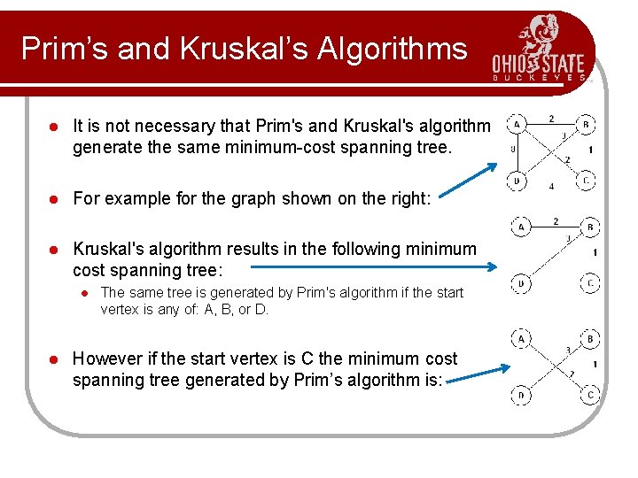
Prim’s and Kruskal’s Algorithms l It is not necessary that Prim's and Kruskal's algorithm generate the same minimum-cost spanning tree. l For example for the graph shown on the right: l Kruskal's algorithm results in the following minimum cost spanning tree: l l The same tree is generated by Prim's algorithm if the start vertex is any of: A, B, or D. However if the start vertex is C the minimum cost spanning tree generated by Prim’s algorithm is:

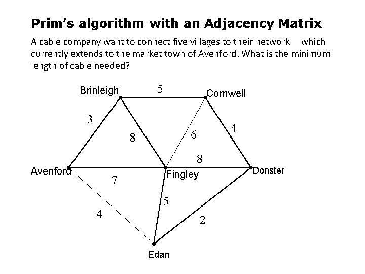
Prim’s algorithm with an Adjacency Matrix A cable company want to connect five villages to their network which currently extends to the market town of Avenford. What is the minimum length of cable needed? 5 Brinleigh Cornwell 3 4 6 8 8 Avenford 7 4 Fingley 5 2 Edan Donster

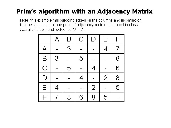
Prim’s algorithm with an Adjacency Matrix Note, this example has outgoing edges on the columns and incoming on the rows, so it is the transpose of adjacency matrix mentioned in class. Actually, it is an undirected, so AT = A. A B C D E F A 3 4 7 B 3 5 8 C 5 4 6 D 4 2 8 E 4 2 5 F 7 8 6 8 5 -

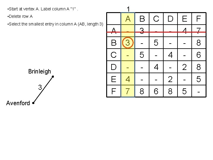
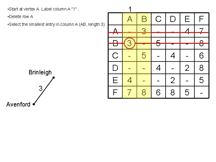
1 • Start at vertex A. Label column A “ 1”. • Delete row A • Select the smallest entry in column A (AB, length 3) Brinleigh 3 Avenford A B C D E F A 3 4 7 B 3 5 8 C D - 5 - 4 4 - 2 6 8 E 4 2 5 F 7 8 6 8 5 -

1 • Start at vertex A. Label column A “ 1”. • Delete row A • Select the smallest entry in column A (AB, length 3) Brinleigh 3 Avenford A B C D E F A 3 4 7 B 3 5 8 C D - 5 - 4 4 - 2 6 8 E 4 2 5 F 7 8 6 8 5 -

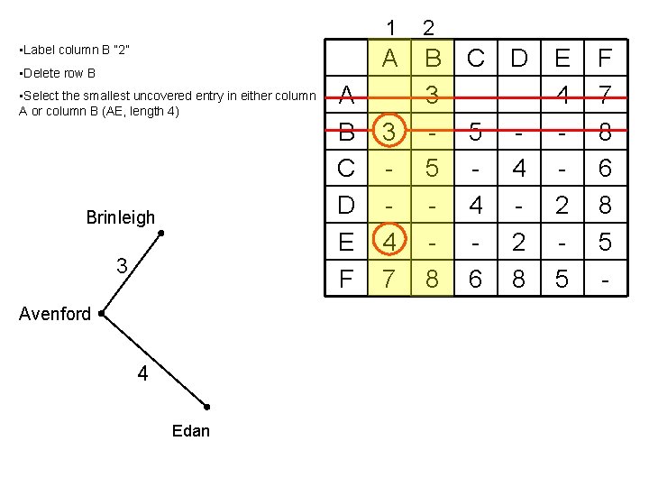
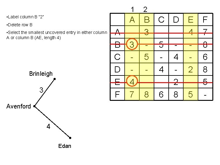
• Label column B “ 2” • Delete row B • Select the smallest uncovered entry in either column A or column B (AE, length 4) Brinleigh 3 Avenford 4 Edan A B C D E F 1 2 A 3 4 7 B 3 5 8 C D - 5 - 4 4 - 2 6 8 E 4 2 5 F 7 8 6 8 5 -

• Label column B “ 2” • Delete row B • Select the smallest uncovered entry in either column A or column B (AE, length 4) Brinleigh 3 Avenford 4 Edan A B C D E F 1 2 A 3 4 7 B 3 5 8 C D - 5 - 4 4 - 2 6 8 E 4 2 5 F 7 8 6 8 5 -

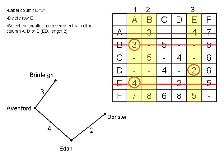
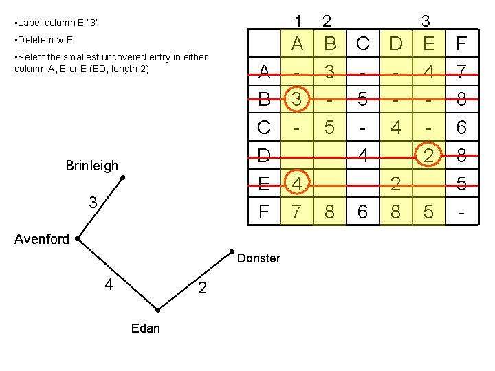
• Label column E “ 3” • Delete row E • Select the smallest uncovered entry in either column A, B or E (ED, length 2) Brinleigh 3 A B C D E F Avenford Donster 4 2 Edan 1 2 A 3 4 7 B 3 5 8 3 C D - 5 - 4 4 - 2 6 8 E 4 2 5 F 7 8 6 8 5 -

• Label column E “ 3” • Delete row E • Select the smallest uncovered entry in either column A, B or E (ED, length 2) Brinleigh 3 A B C D E F Avenford Donster 4 2 Edan 1 2 A 3 4 7 B 3 5 8 3 C D - 5 - 4 4 - 2 6 8 E 4 2 5 F 7 8 6 8 5 -

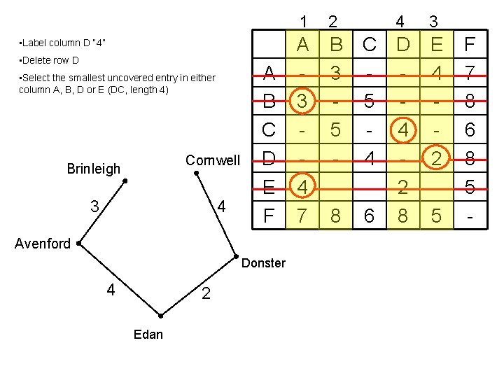
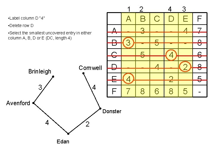
• Label column D “ 4” • Delete row D • Select the smallest uncovered entry in either column A, B, D or E (DC, length 4) Cornwell Brinleigh 4 3 A B C D E F Avenford Donster 4 2 Edan 1 2 A 3 4 7 B 3 5 8 4 C D - 5 - 4 4 - 2 6 8 3 E 4 2 5 F 7 8 6 8 5 -

• Label column D “ 4” • Delete row D • Select the smallest uncovered entry in either column A, B, D or E (DC, length 4) Cornwell Brinleigh 4 3 A B C D E F Avenford Donster 4 2 Edan 1 2 A 3 4 7 B 3 5 8 4 C D - 5 - 4 4 - 2 6 8 3 E 4 2 5 F 7 8 6 8 5 -

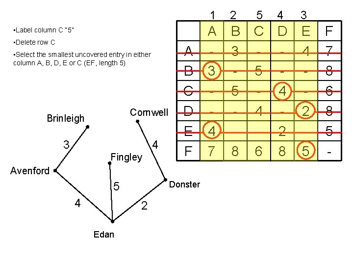
• Label column C “ 5” • Delete row C • Select the smallest uncovered entry in either column A, B, D, E or C (EF, length 5) Cornwell Brinleigh 4 3 Fingley A B C D E F Avenford Donster 5 4 2 Edan 1 2 5 4 A 3 4 7 B 3 5 8 C D - 5 - 4 4 - 2 6 8 3 E 4 2 5 F 7 8 6 8 5 -

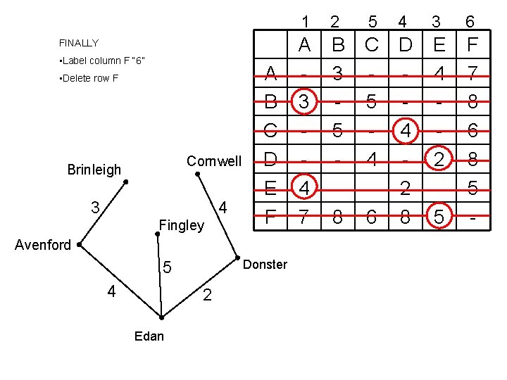
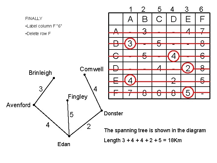
FINALLY • Label column F “ 6” • Delete row F Cornwell Brinleigh 4 3 Fingley A B C D E F Avenford Donster 5 4 2 Edan 1 2 5 4 A 3 4 7 B 3 5 8 C D - 5 - 4 4 - 2 6 8 3 6 E 4 2 5 F 7 8 6 8 5 -

FINALLY • Label column F “ 6” • Delete row F Cornwell Brinleigh 4 3 Fingley A B C D E F 1 2 5 4 A 3 4 7 B 3 5 8 C D - 5 - 4 4 - 2 6 8 3 6 E 4 2 5 F 7 8 6 8 5 - Avenford Donster 5 4 2 Edan The spanning tree is shown in the diagram Length 3 + 4 + 2 + 5 = 18 Km

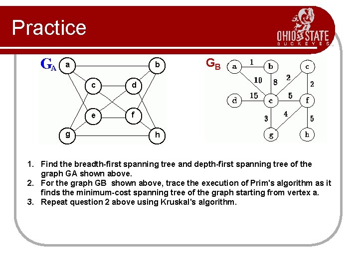
Practice GB 1. Find the breadth-first spanning tree and depth-first spanning tree of the graph GA shown above. 2. For the graph GB shown above, trace the execution of Prim's algorithm as it finds the minimum-cost spanning tree of the graph starting from vertex a. 3. Repeat question 2 above using Kruskal's algorithm.

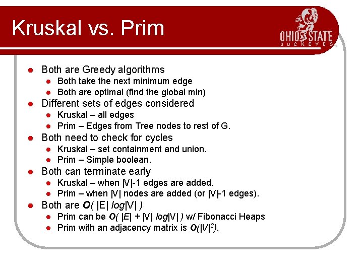
Kruskal vs. Prim l Both are Greedy algorithms l l l Different sets of edges considered l l Kruskal – set containment and union. Prim – Simple boolean. Both can terminate early l l l Kruskal – all edges Prim – Edges from Tree nodes to rest of G. Both need to check for cycles l l Both take the next minimum edge Both are optimal (find the global min) Kruskal – when |V|-1 edges are added. Prim – when |V| nodes are added (or |V|-1 edges). Both are O( |E| log|V| ) l l Prim can be O( |E| + |V| log|V| ) w/ Fibonacci Heaps Prim with an adjacency matrix is O(|V|2).

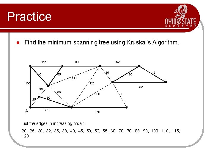
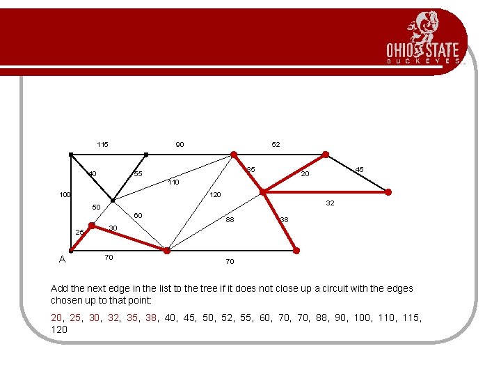
Practice l Find the minimum spanning tree using Kruskal’s Algorithm. 115 90 40 52 35 55 45 20 110 100 120 32 50 60 25 A 88 38 30 70 70 List the edges in increasing order: 20, 25, 30, 32, 35, 38, 40, 45, 50, 52, 55, 60, 70, 88, 90, 100, 115, 120

115 90 40 52 35 55 45 20 110 100 120 32 50 60 25 A 88 38 30 70 70 Starting from the left, add the edge to the tree if it does not close up a circuit with the edges chosen up to that point: 20, 25, 30, 32, 35, 38, 40, 45, 50, 52, 55, 60, 70, 88, 90, 100, 115, 120

115 90 40 52 35 55 45 20 110 100 120 32 50 60 25 A 88 38 30 70 70 Add the next edge in the list to the tree if it does not close up a circuit with the edges chosen up to that point: 20, 25, 30, 32, 35, 38, 40, 45, 50, 52, 55, 60, 70, 88, 90, 100, 115, 120

115 90 40 52 35 55 45 20 110 100 120 32 50 60 25 A 88 38 30 70 70 Add the next edge in the list to the tree if it does not close up a circuit with the edges chosen up to that point: 20, 25, 30, 32, 35, 38, 40, 45, 50, 52, 55, 60, 70, 88, 90, 100, 115, 120

115 90 40 52 35 55 45 20 110 100 120 32 50 60 25 A 88 38 30 70 70 Add the next edge in the list to the tree if it does not close up a circuit with the edges chosen up to that point: 20, 25, 30, 32, 35, 38, 40, 45, 50, 52, 55, 60, 70, 88, 90, 100, 115, 120

115 90 40 52 35 55 45 20 110 100 120 32 50 60 25 A 88 38 30 70 70 Add the next edge in the list to the tree if it does not close up a circuit with the edges chosen up to that point: 20, 25, 30, 32, 35, 38, 40, 45, 50, 52, 55, 60, 70, 88, 90, 100, 115, 120

115 90 40 52 35 55 45 20 110 100 120 32 50 60 25 A 88 38 30 70 70 Add the next edge in the list to the tree if it does not close up a circuit with the edges chosen up to that point: 20, 25, 30, 32, 35, 38, 40, 45, 50, 52, 55, 60, 70, 88, 90, 100, 115, 120

115 90 40 52 35 55 45 20 110 100 120 32 50 60 25 A 88 38 30 70 70 Add the next edge in the list to the tree if it does not close up a circuit with the edges chosen up to that point: 20, 25, 30, 32, 35, 38, 40, 45, 50, 52, 55, 60, 70, 88, 90, 100, 115, 120

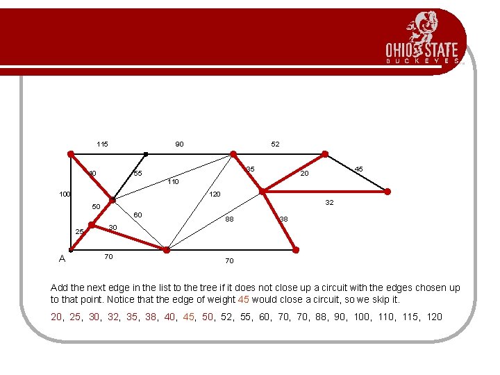
115 90 40 52 35 55 45 20 110 100 120 32 50 60 25 A 88 38 30 70 70 Add the next edge in the list to the tree if it does not close up a circuit with the edges chosen up to that point. Notice that the edge of weight 45 would close a circuit, so we skip it. 20, 25, 30, 32, 35, 38, 40, 45, 50, 52, 55, 60, 70, 88, 90, 100, 115, 120

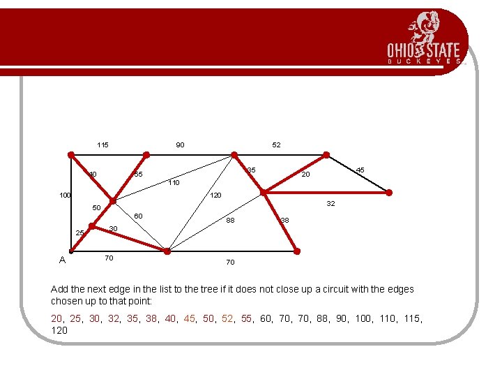
115 90 40 52 35 55 45 20 110 100 120 32 50 60 25 A 88 38 30 70 70 Add the next edge in the list to the tree if it does not close up a circuit with the edges chosen up to that point: 20, 25, 30, 32, 35, 38, 40, 45, 50, 52, 55, 60, 70, 88, 90, 100, 115, 120

115 90 40 52 35 55 45 20 110 100 120 32 50 60 25 A 88 38 30 70 70 Add the next edge in the list to the tree if it does not close up a circuit with the edges chosen up to that point: 20, 25, 30, 32, 35, 38, 40, 45, 50, 52, 55, 60, 70, 88, 90, 100, 115, 120

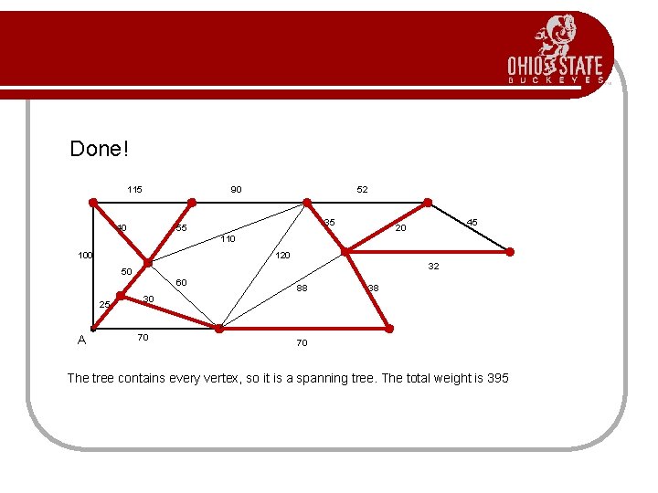
Done! 115 90 40 52 35 55 45 20 110 100 120 32 50 60 25 A 88 38 30 70 70 The tree contains every vertex, so it is a spanning tree. The total weight is 395