Insertion Sort Merge Sort Quick Sort Sorting Problem

Insertion Sort Merge Sort Quick. Sort

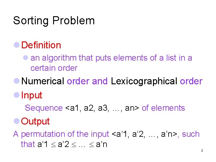
Sorting Problem Definition an algorithm that puts elements of a list in a certain order Numerical order and Lexicographical order Input Sequence <a 1, a 2, a 3, …, an> of elements Output A permutation of the input <a’ 1, a’ 2, …, a’n>, such that a’ 1 a’ 2 … a’n 2

Sorting Problem Two general types of Sorting Internal Sorting, in which all elements are sorted in main memory External Sorting, in which elements must be sorted on disk or tape The focus here is on internal sorting techniques 3

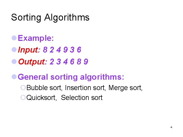
Sorting Algorithms Example: Input: 8 2 4 9 3 6 Output: 2 3 4 6 8 9 General sorting algorithms: Bubble sort, Insertion sort, Merge sort, Quicksort, Selection sort 4

Sorting Algorithms Computational Complexity of element comparisons in terms of the size of the list (N) Recursion recursive or non recursive algorithms Stability stable sorting algorithms maintain the relative order of records with equal keys 5

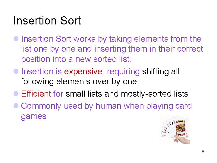
Insertion Sort works by taking elements from the list one by one and inserting them in their correct position into a new sorted list. Insertion is expensive, requiring shifting all following elements over by one Efficient for small lists and mostly-sorted lists Commonly used by human when playing card games 6

Insertion Sort Algorithm we have a n-element sequence and p elements (defined when sorting starts) in the correct order Steps: 1) Initially p = 1. 2) Let the first p elements be sorted. 3) Insert the (p+1)th element properly in the list so that now p+1 elements are sorted. 4) increment p and go to step (2) 7

Example 8

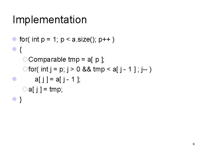
Implementation for( int p = 1; p < a. size(); p++ ) { Comparable tmp = a[ p ]; for( int j = p; j > 0 && tmp < a[ j - 1 ] ; j-- ) a[ j ] = a[ j - 1 ]; a[ j ] = tmp; } 9

Running time Analysis (Best Case) The input is presorted When inserting a[p] into the sorted a[0. . p-1], only need to compare a[p] with a[p-1] and there is no data movement. the test in the inner for loop always fails immediately linear running time O(n) if the input is almost sorted, insertion sort will run quickly 10

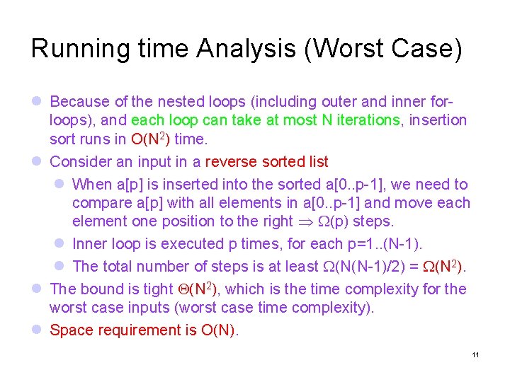
Running time Analysis (Worst Case) Because of the nested loops (including outer and inner forloops), and each loop can take at most N iterations, insertion sort runs in O(N 2) time. Consider an input in a reverse sorted list When a[p] is inserted into the sorted a[0. . p-1], we need to compare a[p] with all elements in a[0. . p-1] and move each element one position to the right (p) steps. Inner loop is executed p times, for each p=1. . (N-1). The total number of steps is at least (N(N-1)/2) = (N 2). The bound is tight (N 2), which is the time complexity for the worst case inputs (worst case time complexity). Space requirement is O(N). 11

Merge Sort and Divide-and-Conquer a classic divide-and-conquer strategy Divide the problem into a number of subproblems (similar to the original problem but smaller) Conquer the sub-problems by solving them recursively (if a sub-problem is small enough, just solve it in a straightforward manner Combine the solutions to the sub-problems into the solution for the original problem 12

Divide-and-Conquer issues Recursion Divide-and-conquer algorithms are naturally implemented as recursive procedures Explicit stack Divide and conquer algorithms can also be implemented by a non-recursive program that stores the partial subproblems in some explicit data structure, such as a stack, queue, or priority queue Sharing repeated sub-problems the branched recursion may end up evaluating the same sub-problem many times over. It may be worth identifying and saving the solutions to overlapping sub-problems 13

Merge Sort Algorithm Step 1 Divide the list into two smaller lists of about equal sizes Step 2 Sort each smaller list recursively Step 3 Merge the two sorted lists to get one sorted list Note: during the recursion, if the subsequence has only one element, then do nothing 14

Dividing Phase Input list is an array A[0. . N-1]. Dividing the array takes O(1) time. We can represent a sublist by two integers left and right: to divide A[left. . Right], we compute center=(left+right)/2 and obtain A[left. . Center] and A[center+1. . Right]. void mergesort(vector<int> & A, int left, int right) { if ( left < right ) { int center = ( left + right ) / 2; mergesort( A, left, center); mergesort( A, center+1, right); merge( A, left, center+1, right); } } 15

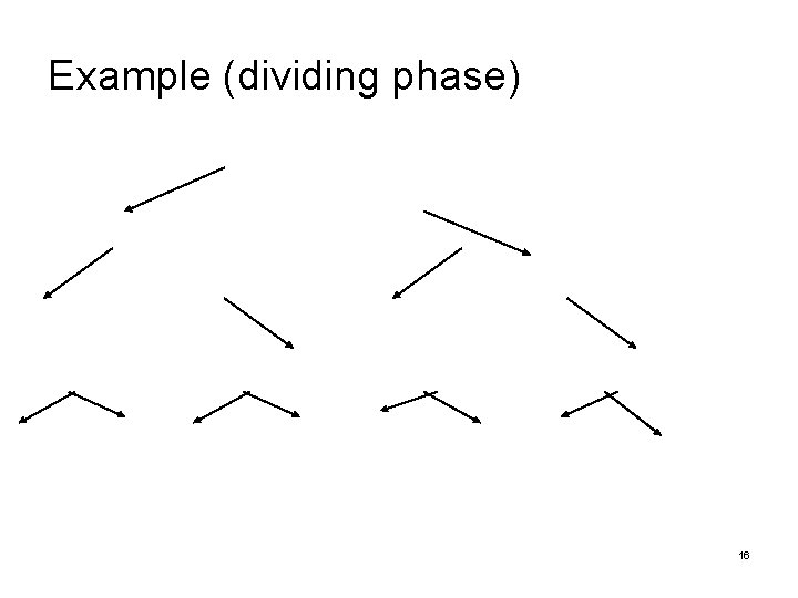
Example (dividing phase) 16

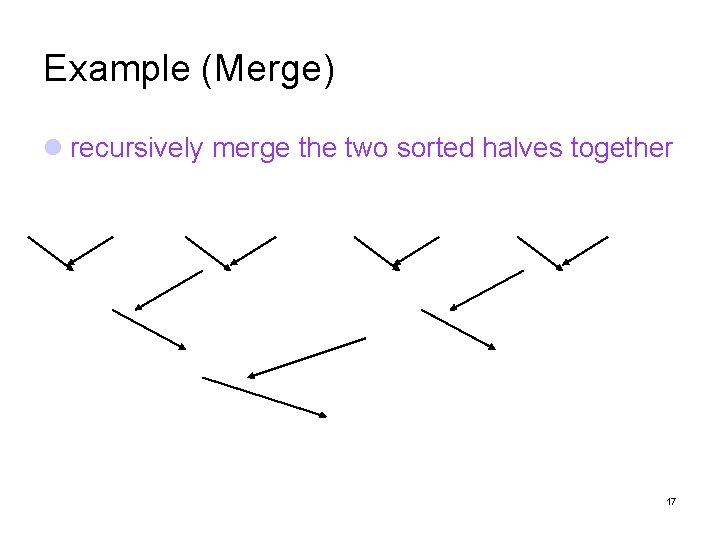
Example (Merge) recursively merge the two sorted halves together 17

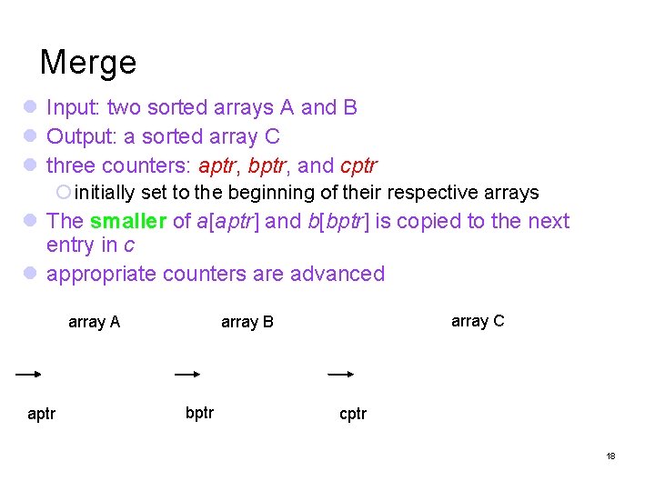
Merge Input: two sorted arrays A and B Output: a sorted array C three counters: aptr, bptr, and cptr initially set to the beginning of their respective arrays The smaller of a[aptr] and b[bptr] is copied to the next entry in c appropriate counters are advanced array A aptr array C array B bptr cptr 18

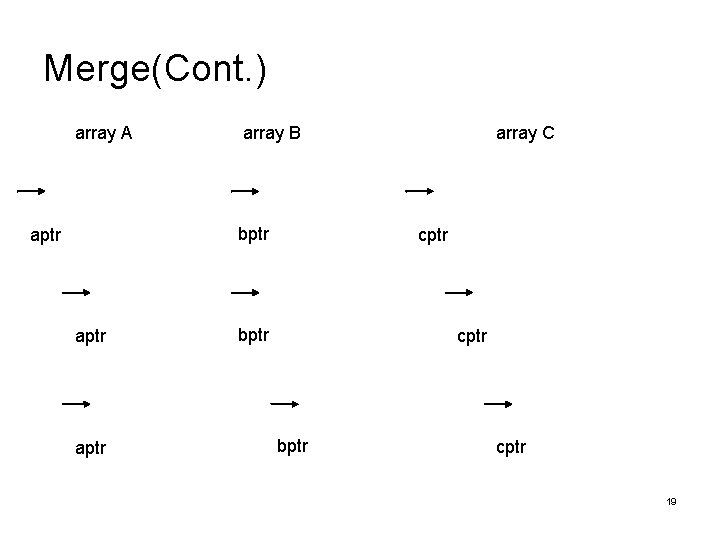
Merge(Cont. ) array A array B bptr aptr array C cptr bptr cptr 19

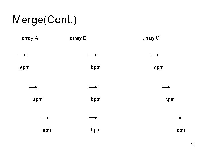
Merge(Cont. ) array A array C array B bptr aptr bptr cptr 20

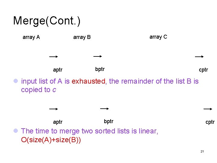
Merge(Cont. ) array A array C array B aptr bptr cptr input list of A is exhausted, the remainder of the list B is copied to c aptr bptr cptr The time to merge two sorted lists is linear, O(size(A)+size(B)) 21

Implementation(Merge) 22

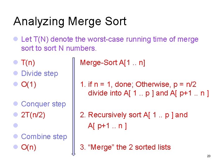
Analyzing Merge Sort Let T(N) denote the worst-case running time of merge sort to sort N numbers. T(n) Divide step O(1) Conquer step 2 T(n/2) Combine step O(n) Merge-Sort A[1. . n] 1. if n = 1, done; Otherwise, p = n/2 divide into A[ 1. . p ] and A[ p+1. . n ] 2. Recursively sort A[ 1. . p ] and A[ p+1. . n ] 3. “Merge” the 2 sorted lists 23

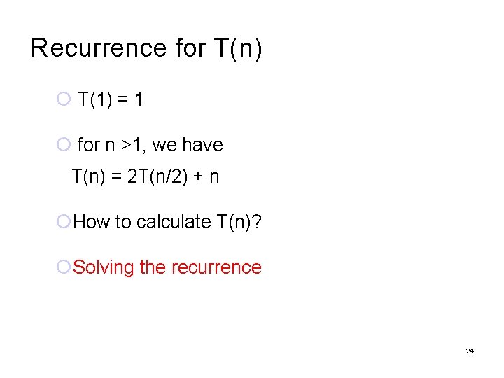
Recurrence for T(n) T(1) = 1 for n >1, we have T(n) = 2 T(n/2) + n How to calculate T(n)? Solving the recurrence 24

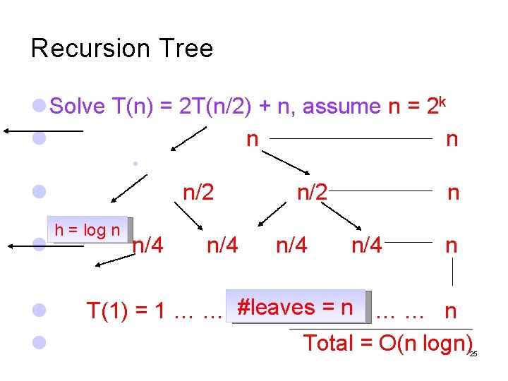
Recursion Tree Solve T(n) = 2 T(n/2) + n, assume n = 2 k n n n/2 h = log n n/4 n/2 n/4 n T(1) = 1 … … #leaves = n … … n Total = O(n logn) 25

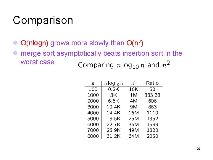
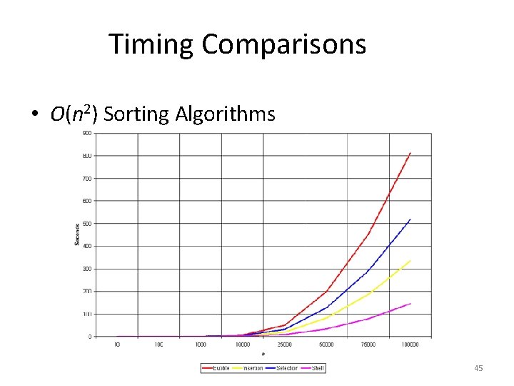
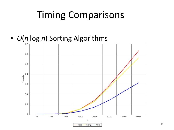
Comparison O(nlogn) grows more slowly than O(n 2) merge sort asymptotically beats insertion sort in the worst case. 26

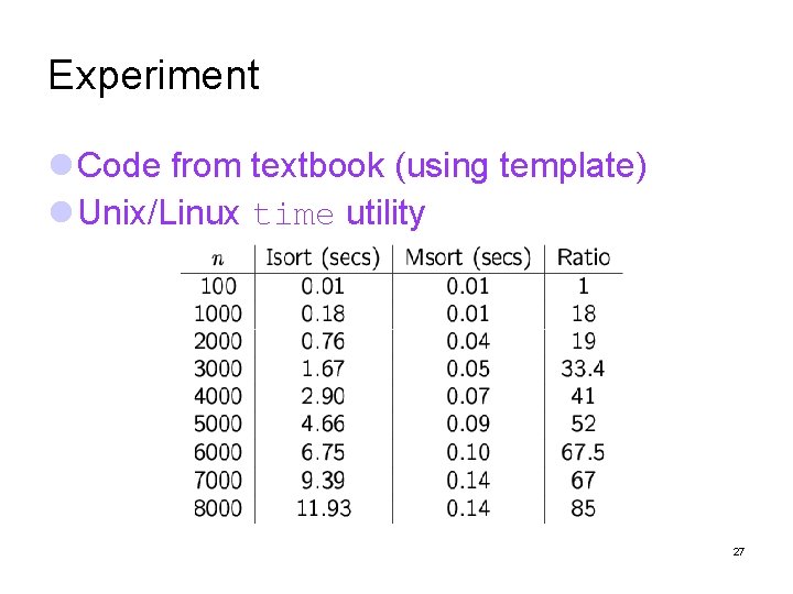
Experiment Code from textbook (using template) Unix/Linux time utility 27

Disadvantage of Merge Sort Space requirement merging two sorted lists requires linear extra memory additional work to copy to the temporary array and back hardly ever used for main memory sorts merging routine is the cornerstone of most external sorting algorithms 28

Quick. Sort Quick. Sort, like merge sort, is based on the divide-and-conquer recursive algorithm Fastest known sorting algorithm in practice Best case running time: O(N log N) Worst case running time: O(N 2) But, the worst case seldom happens

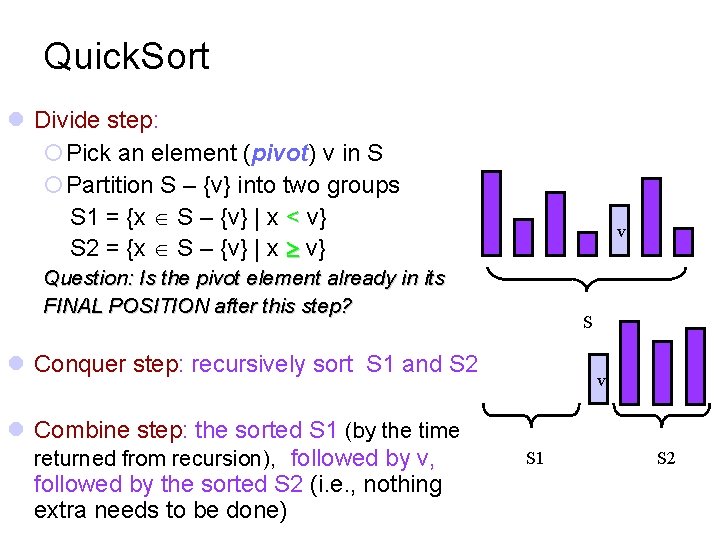
Quick. Sort Divide step: Pick an element (pivot) v in S Partition S – {v} into two groups S 1 = {x S – {v} | x < v} S 2 = {x S – {v} | x v} v Question: Is the pivot element already in its FINAL POSITION after this step? S Conquer step: recursively sort S 1 and S 2 Combine step: the sorted S 1 (by the time returned from recursion), followed by v, followed by the sorted S 2 (i. e. , nothing extra needs to be done) v S 1 S 2

Pseudocode Input: an array A[p, r] Quicksort (A, p, r) { Divide if (p < r) { q = Partition (A, p, r) //q is the position of the pivot element Quicksort (A, p, q-1) Quicksort (A, q+1, r) } } Conquer

Two main problems Problem 1: How to choose the pivot element in each step? Problem 2: If the pivot element is chosen, how to perform the partition?

Problem 2: Partition Key step of the quicksort algorithm Let’s say we want to sort an array A[p: : r]. Assume that We select x = A[q] as a pivot. Then how can we partition the array into two Segments S 1, S 2?

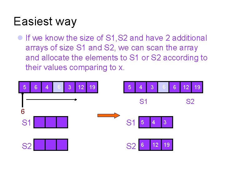
Easiest way If we know the size of S 1, S 2 and have 2 additional arrays of size S 1 and S 2, we can scan the array and allocate the elements to S 1 or S 2 according to their values comparing to x. 5 6 4 6 3 12 19 5 4 3 6 S 1 6 12 19 S 2 6 S 1 5 4 S 2 6 12 19 3

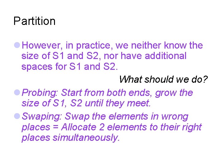
Partition However, in practice, we neither know the size of S 1 and S 2, nor have additional spaces for S 1 and S 2. What should we do? Probing: Start from both ends, grow the size of S 1, S 2 until they meet. Swaping: Swap the elements in wrong places = Allocate 2 elements to their right places simultaneously.

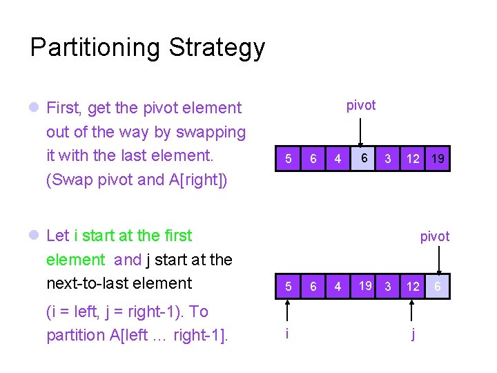
Partitioning Strategy First, get the pivot element out of the way by swapping it with the last element. (Swap pivot and A[right]) Let i start at the first element and j start at the next-to-last element (i = left, j = right-1). To partition A[left … right-1]. pivot 5 6 4 6 3 12 19 pivot 5 i 6 4 19 3 12 j 6

Partitioning Strategy Two Requirements: A[p] <= pivot, for p < i A[p] >= pivot, for p > j <=pivot >=pivot i j When i < j Move i right, skipping over elements smaller than the pivot (In other words, move i right, compare, stop when A[i] >= pivot). Move j left, skipping over elements greater than the pivot (In other wards, move j left, compare, stop when A[j] <= pivot or j is out of range).

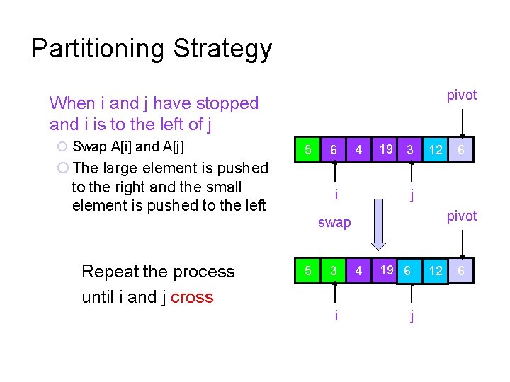
Partitioning Strategy pivot When i and j have stopped and i is to the left of j Swap A[i] and A[j] 5 The large element is pushed to the right and the small element is pushed to the left 6 4 i 19 3 12 j pivot swap Repeat the process until i and j cross 5 3 i 6 4 19 6 j 12 6

Partitioning Strategy pivot When i and j have crossed 5 3 4 Swap A[i] and pivot, where A[i] >= pivot. 19 6 12 6 6 12 19 j < i swap Results: A[p] <= pivot, for p < i A[p] >= pivot, for p > i 5 3 4 6 j i

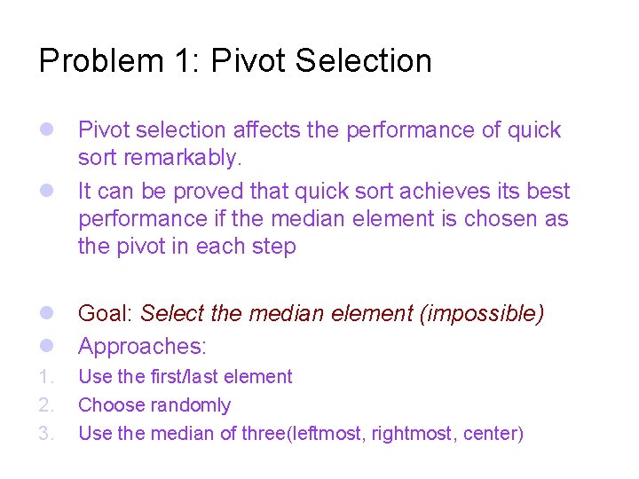
Problem 1: Pivot Selection Pivot selection affects the performance of quick sort remarkably. It can be proved that quick sort achieves its best performance if the median element is chosen as the pivot in each step Goal: Select the median element (impossible) Approaches: 1. 2. 3. Use the first/last element Choose randomly Use the median of three(leftmost, rightmost, center)

Pseudocode of Quick Sort void quicksort(A[], p, r) { int i = p; int j = r-1; if(i <= j) { int pivot = A[r]; // pick the rightmost element as pivot //begin partitioning for(; ; ) { while(A[i]<pivot && i<r) { i++; } while(A[j]>pivot && j>p) { j--; } if(i < j) swap(A[i], A[j]); else break; } swap(A[i], A[r]); // recursive sort each partition quicksort(A, p, i-1); // Sort left partition quicksort(A, i+1, r); // Sort right partition } }

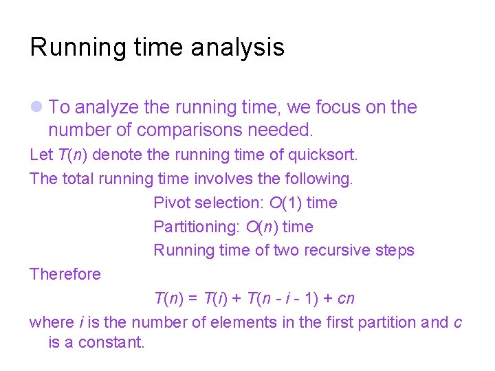
Running time analysis To analyze the running time, we focus on the number of comparisons needed. Let T(n) denote the running time of quicksort. The total running time involves the following. Pivot selection: O(1) time Partitioning: O(n) time Running time of two recursive steps Therefore T(n) = T(i) + T(n - i - 1) + cn where i is the number of elements in the first partition and c is a constant.

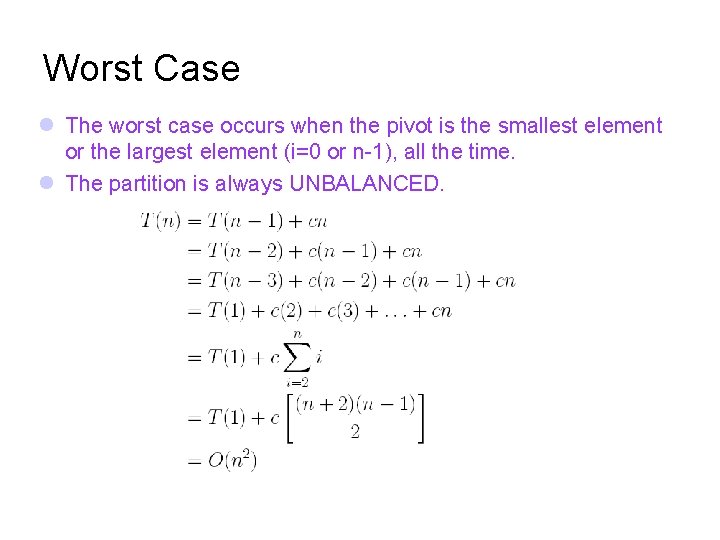
Worst Case The worst case occurs when the pivot is the smallest element or the largest element (i=0 or n-1), all the time. The partition is always UNBALANCED.

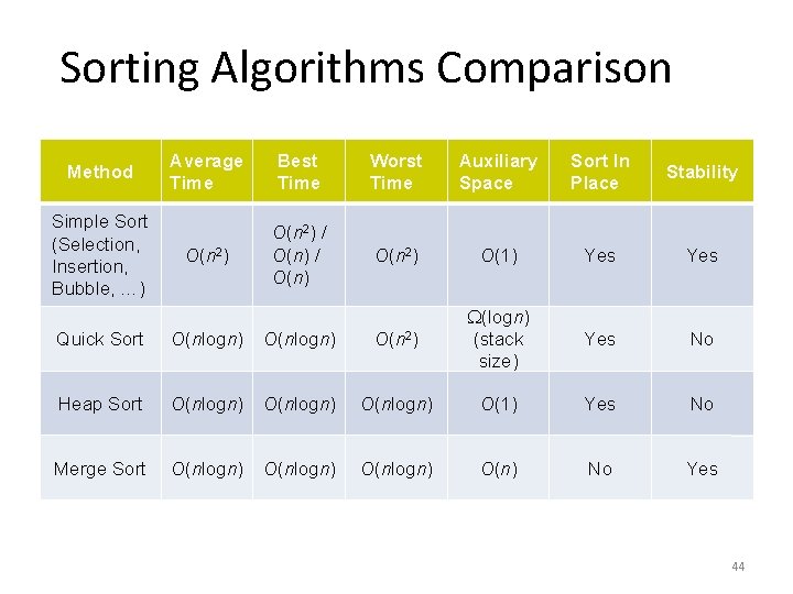
Sorting Algorithms Comparison Method Simple Sort (Selection, Insertion, Bubble, …) Average Time Best Time Worst Time Auxiliary Space Sort In Place Stability O(n 2) / O(n) O(n 2) O(1) Yes Yes No Quick Sort O(nlogn) O(n 2) (logn) (stack size) Heap Sort O(nlogn) O(1) Yes No Merge Sort O(nlogn) O(n) No Yes 44

Timing Comparisons • O(n 2) Sorting Algorithms 45

Timing Comparisons • O(n log n) Sorting Algorithms 46

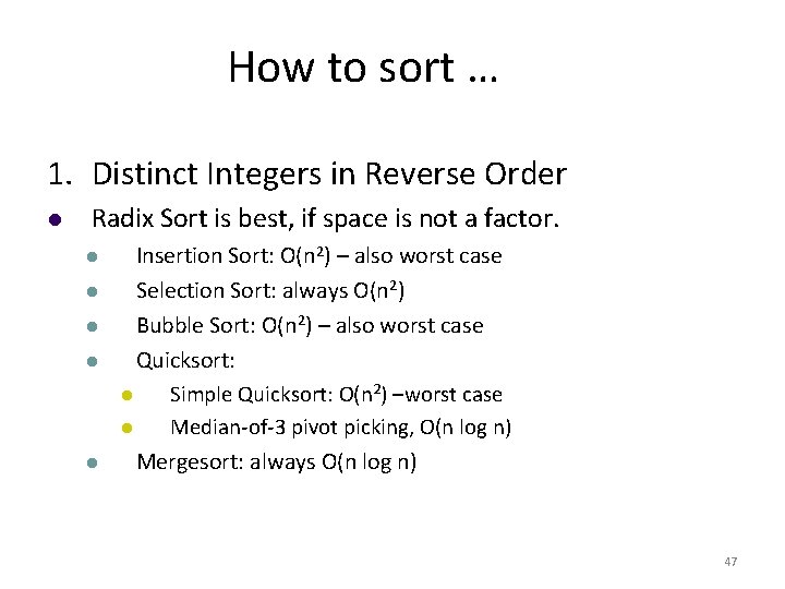
How to sort … 1. Distinct Integers in Reverse Order Radix Sort is best, if space is not a factor. Insertion Sort: O(n 2) – also worst case Selection Sort: always O(n 2) Bubble Sort: O(n 2) – also worst case Quicksort: Simple Quicksort: O(n 2) –worst case Median-of-3 pivot picking, O(n log n) Mergesort: always O(n log n) 47

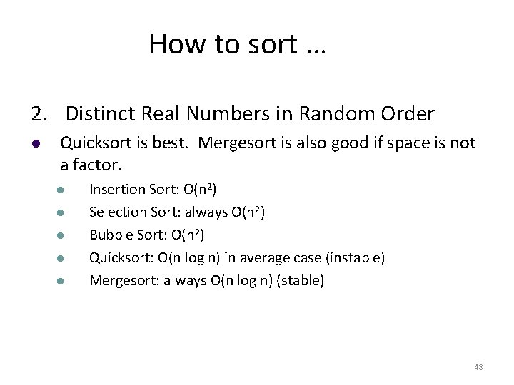
How to sort … 2. Distinct Real Numbers in Random Order Quicksort is best. Mergesort is also good if space is not a factor. Insertion Sort: O(n 2) Selection Sort: always O(n 2) Bubble Sort: O(n 2) Quicksort: O(n log n) in average case (instable) Mergesort: always O(n log n) (stable) 48

How to sort … 1. Distinct Integers with One Element Out of Place Insertion Sort is best. If the element is “later” than its proper place then Bubble Sort (to the smallest end) is also good. 49

How to sort … 3. Distinct Integers with One Element Out of Place Insertion Sort: O(n) Selection Sort: always O(n 2) Bubble Sort: “Later”: O(n). “Earlier”: O(n 2). Quicksort: Simple Quicksort: O(n 2) –close to the worst case Median-of-3 pivot picking, O(n log n) Mergesort: always O(n log n) 50

How to sort … 4. Distinct Real Numbers, “Almost Sorted” Insertion Sort is best, Bubble Sort almost as good Insertion Sort: Almost O(n). Selection Sort: always O(n 2) Bubble Sort: Almost O(n). Quicksort: depending on data, somewhere between O(n 2) and O(n log n) Mergesort: always O(n log n) 51