Sorting Gordon College 1 Sorting Consider a list

Sorting Gordon College 1

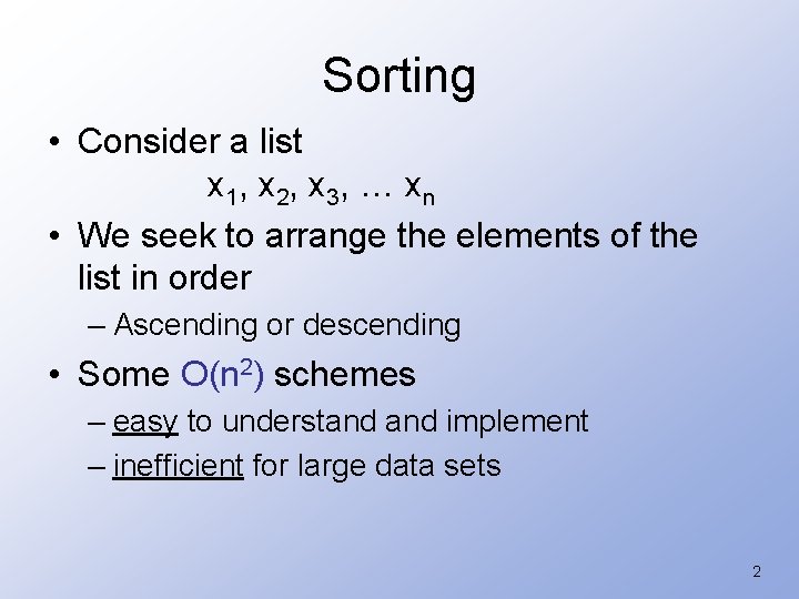
Sorting • Consider a list x 1, x 2, x 3, … xn • We seek to arrange the elements of the list in order – Ascending or descending • Some O(n 2) schemes – easy to understand implement – inefficient for large data sets 2

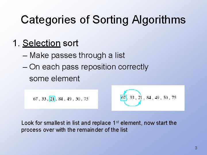
Categories of Sorting Algorithms 1. Selection sort – Make passes through a list – On each pass reposition correctly some element Look for smallest in list and replace 1 st element, now start the process over with the remainder of the list 3

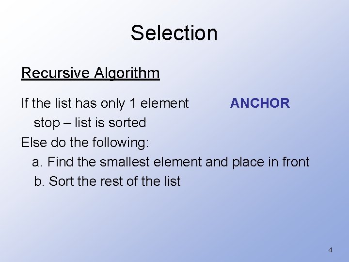
Selection Recursive Algorithm If the list has only 1 element ANCHOR stop – list is sorted Else do the following: a. Find the smallest element and place in front b. Sort the rest of the list 4

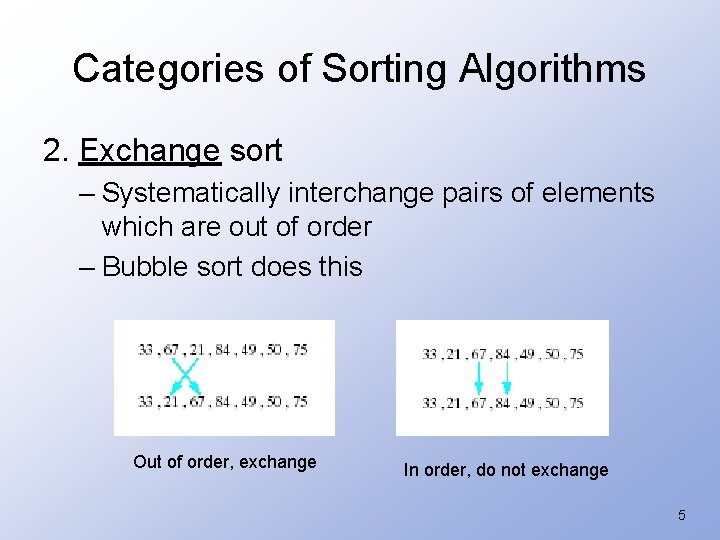
Categories of Sorting Algorithms 2. Exchange sort – Systematically interchange pairs of elements which are out of order – Bubble sort does this Out of order, exchange In order, do not exchange 5

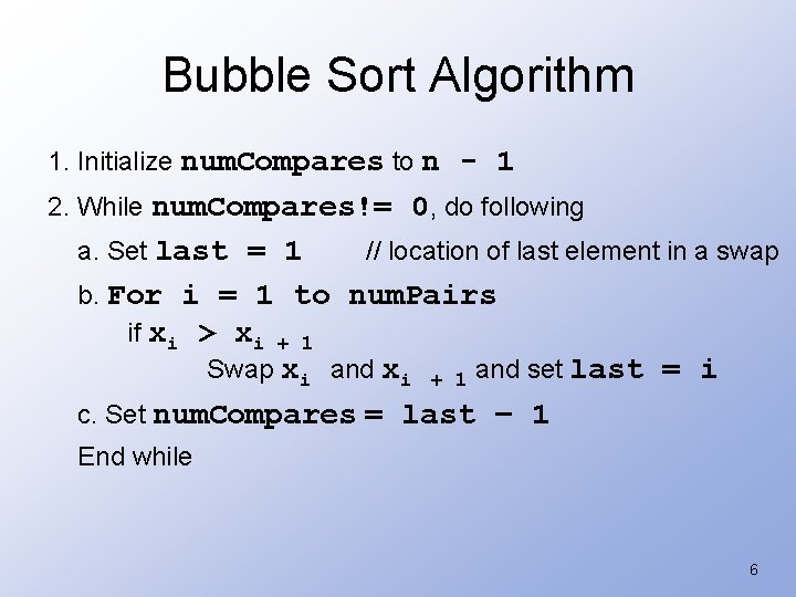
Bubble Sort Algorithm 1. Initialize num. Compares to n - 1 2. While num. Compares!= 0, do following a. Set last = 1 // location of last element in a swap b. For i = 1 to num. Pairs if xi > xi + 1 Swap xi and xi + 1 and set last = i c. Set num. Compares = last – 1 End while 6

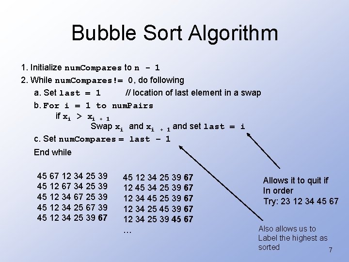
Bubble Sort Algorithm 1. Initialize num. Compares to n - 1 2. While num. Compares!= 0, do following a. Set last = 1 // location of last element in a swap b. For i = 1 to num. Pairs if xi > xi + 1 Swap xi and xi + 1 and set last = i c. Set num. Compares = last – 1 End while 45 67 12 34 25 39 45 12 67 34 25 39 45 12 34 67 25 39 45 12 34 25 67 39 45 12 34 25 39 67 12 45 34 25 39 67 12 34 45 25 39 67 12 34 25 45 39 67 12 34 25 39 45 67 … Allows it to quit if In order Try: 23 12 34 45 67 Also allows us to Label the highest as sorted 7

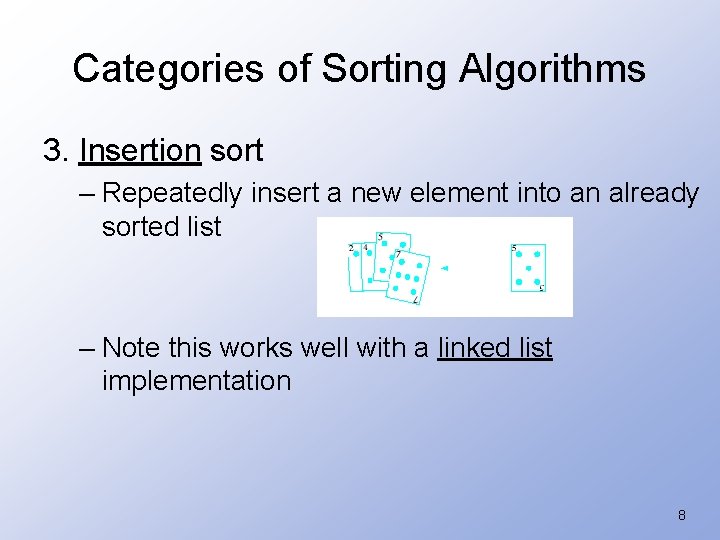
Categories of Sorting Algorithms 3. Insertion sort – Repeatedly insert a new element into an already sorted list – Note this works well with a linked list implementation 8

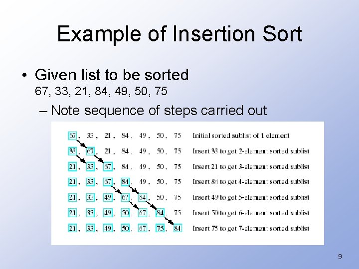
Example of Insertion Sort • Given list to be sorted 67, 33, 21, 84, 49, 50, 75 – Note sequence of steps carried out 9

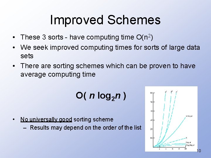
Improved Schemes • These 3 sorts - have computing time O(n 2) • We seek improved computing times for sorts of large data sets • There are sorting schemes which can be proven to have average computing time O( n log 2 n ) • No universally good sorting scheme – Results may depend on the order of the list 10

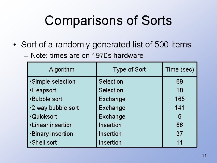
Comparisons of Sorts • Sort of a randomly generated list of 500 items – Note: times are on 1970 s hardware Algorithm • Simple selection • Heapsort • Bubble sort • 2 way bubble sort • Quicksort • Linear insertion • Binary insertion • Shell sort Type of Sort Selection Exchange Insertion Time (sec) 69 18 165 141 6 66 37 11 11

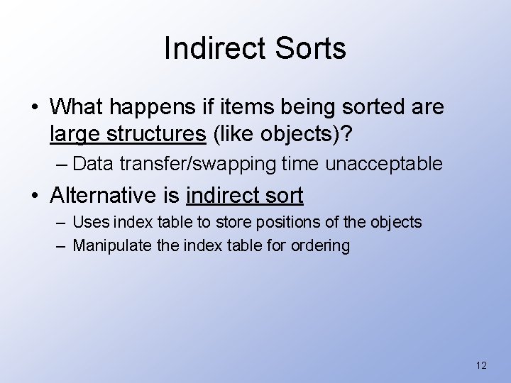
Indirect Sorts • What happens if items being sorted are large structures (like objects)? – Data transfer/swapping time unacceptable • Alternative is indirect sort – Uses index table to store positions of the objects – Manipulate the index table for ordering 12

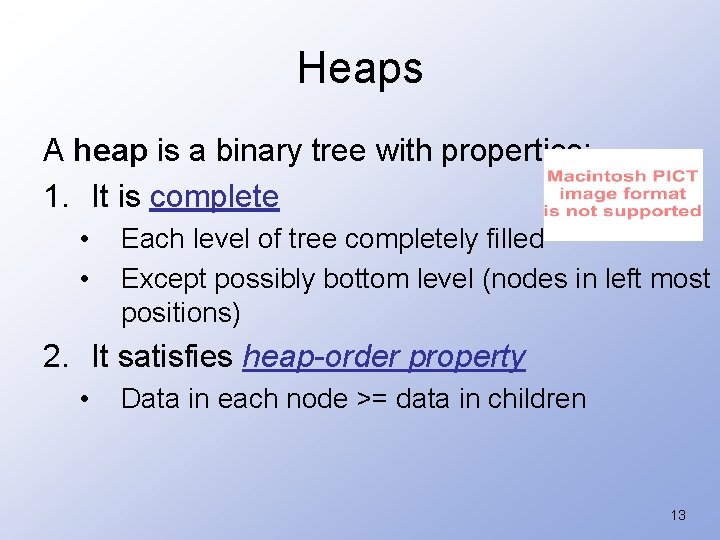
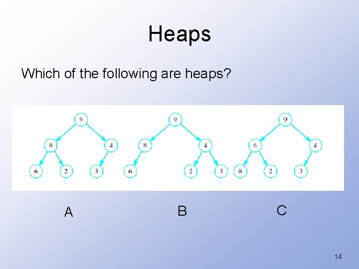
Heaps A heap is a binary tree with properties: 1. It is complete • • Each level of tree completely filled Except possibly bottom level (nodes in left most positions) 2. It satisfies heap-order property • Data in each node >= data in children 13

Heaps Which of the following are heaps? A B C 14

Maximum and Minimum Heaps Example 15

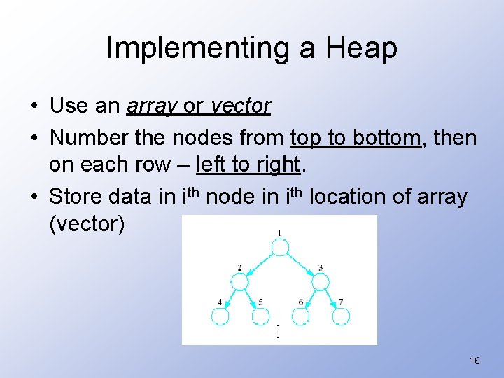
Implementing a Heap • Use an array or vector • Number the nodes from top to bottom, then on each row – left to right. • Store data in ith node in ith location of array (vector) 16

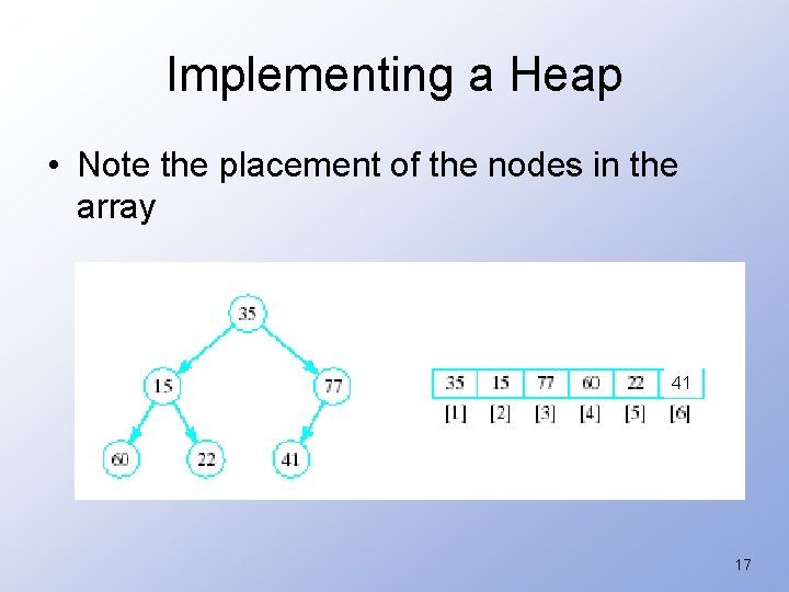
Implementing a Heap • Note the placement of the nodes in the array 41 17

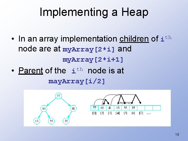
Implementing a Heap • In an array implementation children of ith node are at my. Array[2*i] and my. Array[2*i+1] • Parent of the ith node is at may. Array[i/2] 18

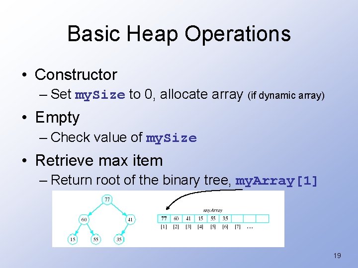
Basic Heap Operations • Constructor – Set my. Size to 0, allocate array (if dynamic array) • Empty – Check value of my. Size • Retrieve max item – Return root of the binary tree, my. Array[1] 19

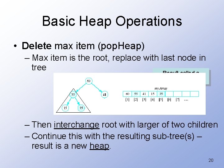
Basic Heap Operations • Delete max item (pop. Heap) – Max item is the root, replace with last node in tree Result called a semiheap – Then interchange root with larger of two children – Continue this with the resulting sub-tree(s) – result is a new heap. 20

Exchanging elements when performing a pop. Heap() 21

Adjusting the heap for pop. Heap() 22

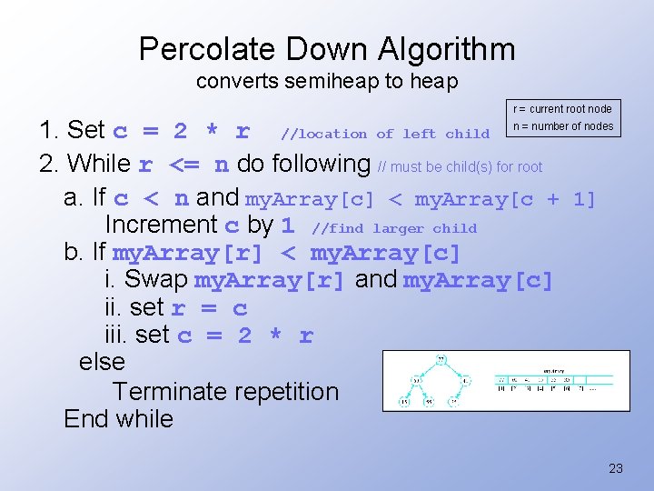
Percolate Down Algorithm converts semiheap to heap r = current root node 1. Set c = 2 * r //location of left child n = number of nodes 2. While r <= n do following // must be child(s) for root a. If c < n and my. Array[c] < my. Array[c + 1] Increment c by 1 //find larger child b. If my. Array[r] < my. Array[c] i. Swap my. Array[r] and my. Array[c] ii. set r = c iii. set c = 2 * r else Terminate repetition End while 23

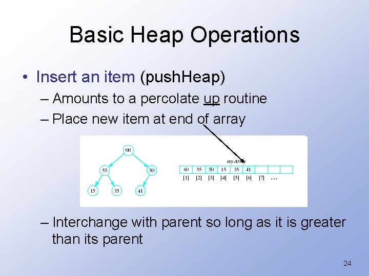
Basic Heap Operations • Insert an item (push. Heap) – Amounts to a percolate up routine – Place new item at end of array – Interchange with parent so long as it is greater than its parent 24

Example of Heap Before and After Insertion of 50 25

Reordering the tree for the insertion 26

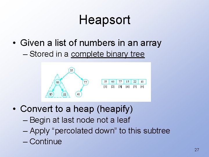
Heapsort • Given a list of numbers in an array – Stored in a complete binary tree • Convert to a heap (heapify) – Begin at last node not a leaf – Apply “percolated down” to this subtree – Continue 27

Example of Heapifying a Vector 28

Example of Heapifying a Vector 29

Example of Heapifying a Vector 30

Example of Heapifying a Vector 31

Example of Heapifying a Vector 32

Example of Heapifying a Vector 33

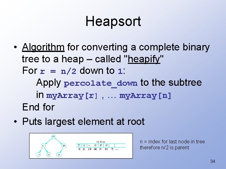
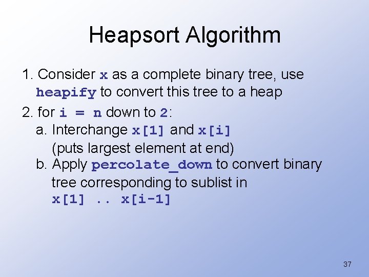
Heapsort • Algorithm for converting a complete binary tree to a heap – called "heapify" For r = n/2 down to 1: Apply percolate_down to the subtree in my. Array[r] , … my. Array[n] End for • Puts largest element at root n = index for last node in tree therefore n/2 is parent 34

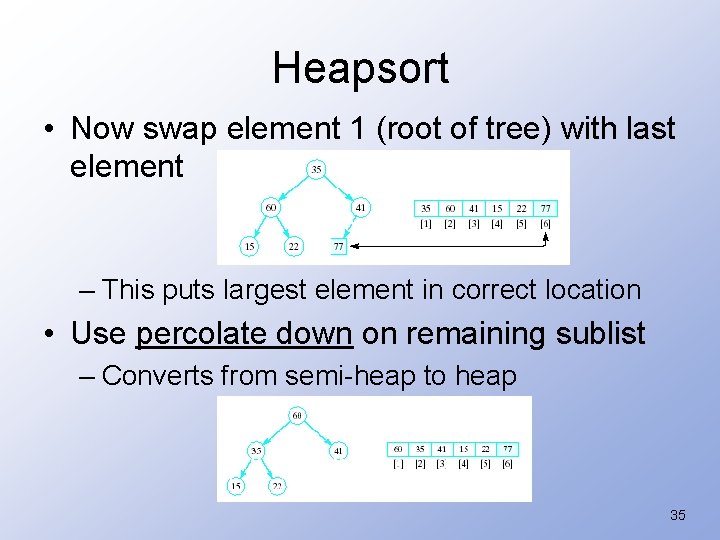
Heapsort • Now swap element 1 (root of tree) with last element – This puts largest element in correct location • Use percolate down on remaining sublist – Converts from semi-heap to heap 35

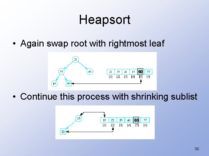
Heapsort • Again swap root with rightmost leaf 60 • Continue this process with shrinking sublist 60 36

Heapsort Algorithm 1. Consider x as a complete binary tree, use heapify to convert this tree to a heap 2. for i = n down to 2: a. Interchange x[1] and x[i] (puts largest element at end) b. Apply percolate_down to convert binary tree corresponding to sublist in x[1]. . x[i-1] 37

Example of Implementing heap sort int arr[] = {50, 20, 75, 35, 25}; vector<int> v(arr, 5); 38

Example of Implementing heap sort 39

Example of Implementing heap sort 40

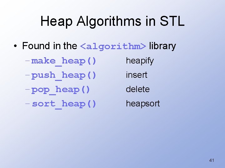
Heap Algorithms in STL • Found in the <algorithm> library – make_heap() heapify – push_heap() insert – pop_heap() delete – sort_heap() heapsort 41

Priority Queue • A collection of data elements – Items stored in order by priority – Higher priority items removed ahead of lower Implementation ? 42

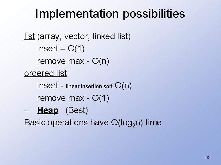
Implementation possibilities list (array, vector, linked list) insert – O(1) remove max - O(n) ordered list insert - linear insertion sort O(n) remove max - O(1) – Heap (Best) Basic operations have O(log 2 n) time 43

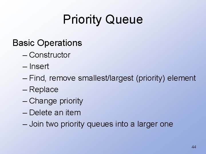
Priority Queue Basic Operations – Constructor – Insert – Find, remove smallest/largest (priority) element – Replace – Change priority – Delete an item – Join two priority queues into a larger one 44

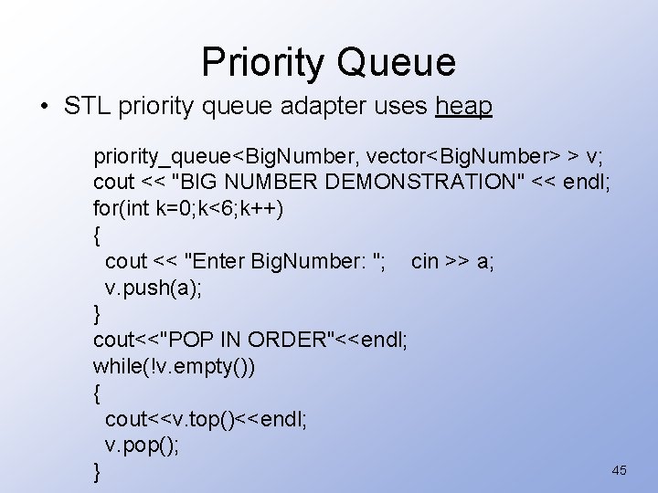
Priority Queue • STL priority queue adapter uses heap priority_queue<Big. Number, vector<Big. Number> > v; cout << "BIG NUMBER DEMONSTRATION" << endl; for(int k=0; k<6; k++) { cout << "Enter Big. Number: "; cin >> a; v. push(a); } cout<<"POP IN ORDER"<<endl; while(!v. empty()) { cout<<v. top()<<endl; v. pop(); 45 }

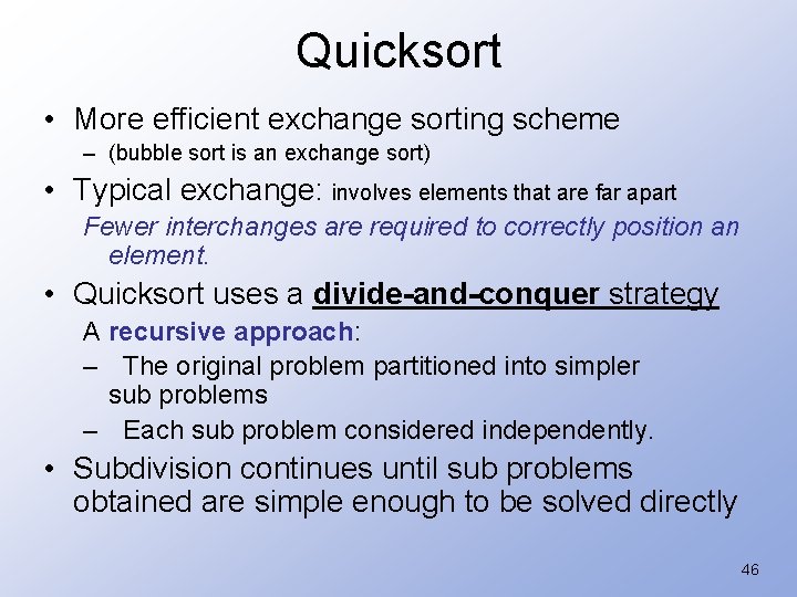
Quicksort • More efficient exchange sorting scheme – (bubble sort is an exchange sort) • Typical exchange: involves elements that are far apart Fewer interchanges are required to correctly position an element. • Quicksort uses a divide-and-conquer strategy A recursive approach: – The original problem partitioned into simpler sub problems – Each sub problem considered independently. • Subdivision continues until sub problems obtained are simple enough to be solved directly 46

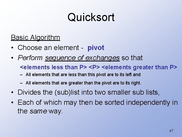
Quicksort Basic Algorithm • Choose an element - pivot • Perform sequence of exchanges so that <elements less than P> <elements greater than P> – All elements that are less than this pivot are to its left and – All elements that are greater than the pivot are to its right. • Divides the (sub)list into two smaller sub lists, • Each of which may then be sorted independently in the same way. 47

Quicksort recursive If the list has 0 or 1 elements, ANCHOR return. // the list is sorted Else do: Pick an element in the list to use as the pivot. Split the remaining elements into two disjoint groups: Smaller. Than. Pivot = {all elements < pivot} Larger. Than. Pivot = {all elements > pivot} Return the list rearranged as: Quicksort(Smaller. Than. Pivot), pivot, Quicksort(Larger. Than. Pivot). 48

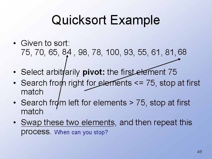
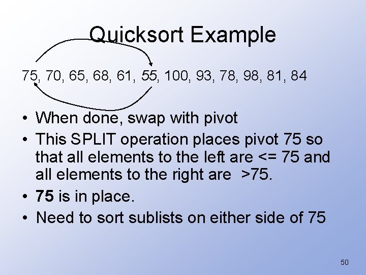
Quicksort Example • Given to sort: 84 68 75, 70, 65, , 98, 78, 100, 93, 55, 61, 81, • Select arbitrarily pivot: the first element 75 • Search from right for elements <= 75, stop at first match • Search from left for elements > 75, stop at first match • Swap these two elements, and then repeat this process. When can you stop? 49

Quicksort Example 75, 70, 65, 68, 61, 55, 100, 93, 78, 98, 81, 84 • When done, swap with pivot • This SPLIT operation places pivot 75 so that all elements to the left are <= 75 and all elements to the right are >75. • 75 is in place. • Need to sort sublists on either side of 75 50

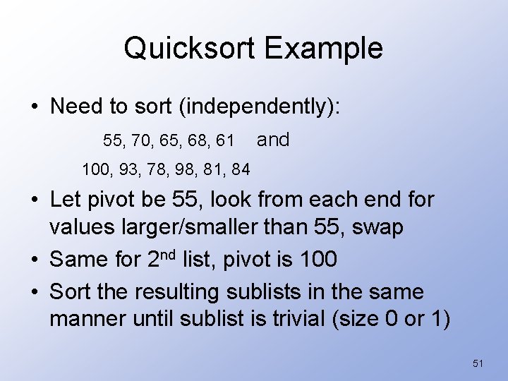
Quicksort Example • Need to sort (independently): 55, 70, 65, 68, 61 and 100, 93, 78, 98, 81, 84 • Let pivot be 55, look from each end for values larger/smaller than 55, swap • Same for 2 nd list, pivot is 100 • Sort the resulting sublists in the same manner until sublist is trivial (size 0 or 1) 51

Quick. Sort Recursive Function template <typename Element. Type> void quicksort (Element. Type x[], int first int last) { int pos; // pivot's final position if (first < last) // list size is > 1 { split(x, first, last, pos); // Split into 2 sublists quicksort(x, first, pos - 1); // Sort left sublist quicksort(x, pos + 1, last); // Sort right sublist } } 23 45 12 67 32 56 90 2 15 52

template <typename Element. Type> void split (Element. Type x[], int first, int last, int & pos) { Element. Type pivot = x[first]; // pivot element int left = first, // index for left search right = last; // index for right search while (left < right) { while (pivot < x[right]) // Search from right for right--; // element <= pivot // Search from left for while (left < right && // element > pivot x[left] <= pivot) left++; if (left < right) // If searches haven't met swap (x[left], x[right]); // interchange elements } // End of searches; place pivot in correct position pos = right; x[first] = x[pos]; 23 45 12 67 32 56 90 2 15 x[pos] = pivot; } 53

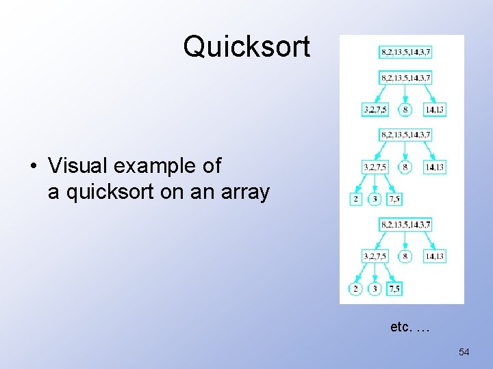
Quicksort • Visual example of a quicksort on an array etc. … 54

Quick. Sort Example v = {800, 150, 300, 650, 500, 400, 350, 450, 900} Pivot selected at random 55

Quick. Sort Example 56

Quick. Sort Example 57

Quick. Sort Example 58

Quick. Sort Example quicksort(x, 0, 4); quicksort(x, 6, 9); 59

Quick. Sort Example quicksort(x, 0, 0); quicksort(x, 2, 4); 60

Quick. Sort Example quicksort(x, 6, 6); quicksort(x, 8, 9); 61

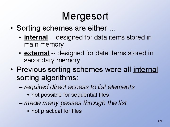
Quick. Sort Example 62

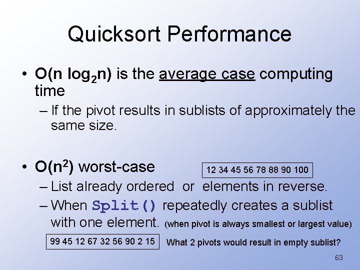
Quicksort Performance • O(n log 2 n) is the average case computing time – If the pivot results in sublists of approximately the same size. • O(n 2) worst-case 12 34 45 56 78 88 90 100 – List already ordered or elements in reverse. – When Split() repeatedly creates a sublist with one element. (when pivot is always smallest or largest value) 99 45 12 67 32 56 90 2 15 What 2 pivots would result in empty sublist? 63

Improvements to Quicksort 12 34 45 56 78 88 90 100 • An arbitrary pivot gives a poor partition for nearly sorted lists (or lists in reverse) • Virtually all the elements go into either Smaller. Than. Pivot or Larger. Than. Pivot – all through the recursive calls. • Quicksort takes quadratic time to do essentially nothing at all. 64

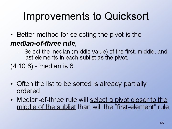
Improvements to Quicksort • Better method for selecting the pivot is the median-of-three rule, – Select the median (middle value) of the first, middle, and last elements in each sublist as the pivot. (4 10 6) - median is 6 • Often the list to be sorted is already partially ordered • Median-of-three rule will select a pivot closer to the middle of the sublist than will the “first-element” rule. 65

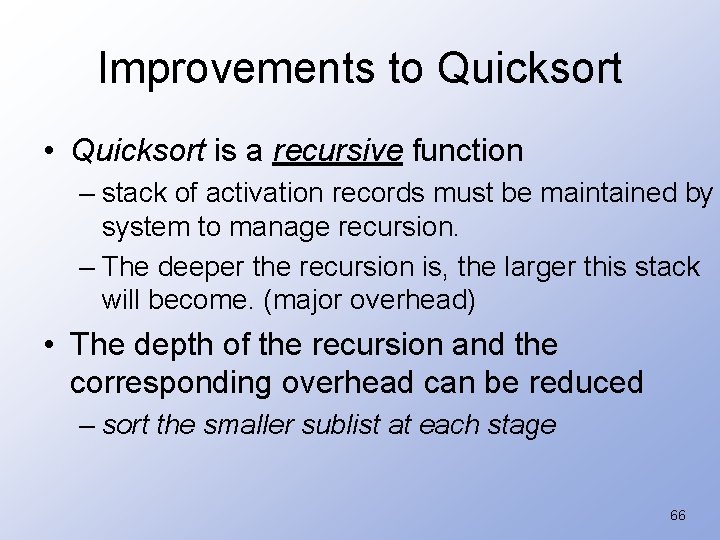
Improvements to Quicksort • Quicksort is a recursive function – stack of activation records must be maintained by system to manage recursion. – The deeper the recursion is, the larger this stack will become. (major overhead) • The depth of the recursion and the corresponding overhead can be reduced – sort the smaller sublist at each stage 66

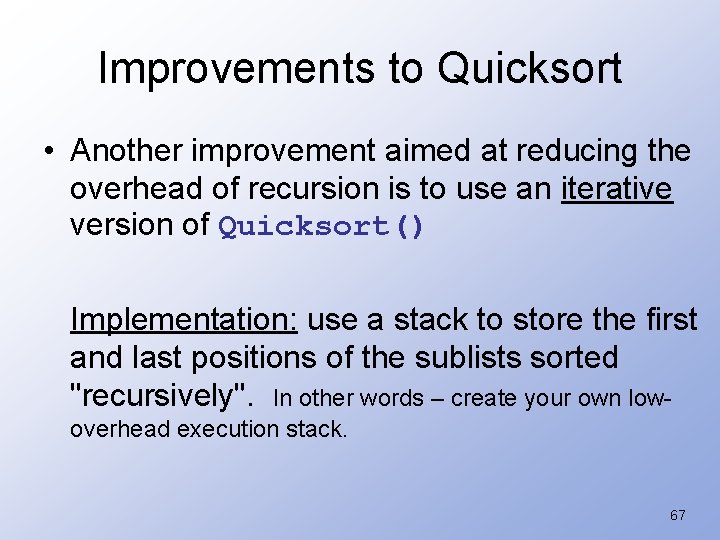
Improvements to Quicksort • Another improvement aimed at reducing the overhead of recursion is to use an iterative version of Quicksort() Implementation: use a stack to store the first and last positions of the sublists sorted "recursively". In other words – create your own lowoverhead execution stack. 67

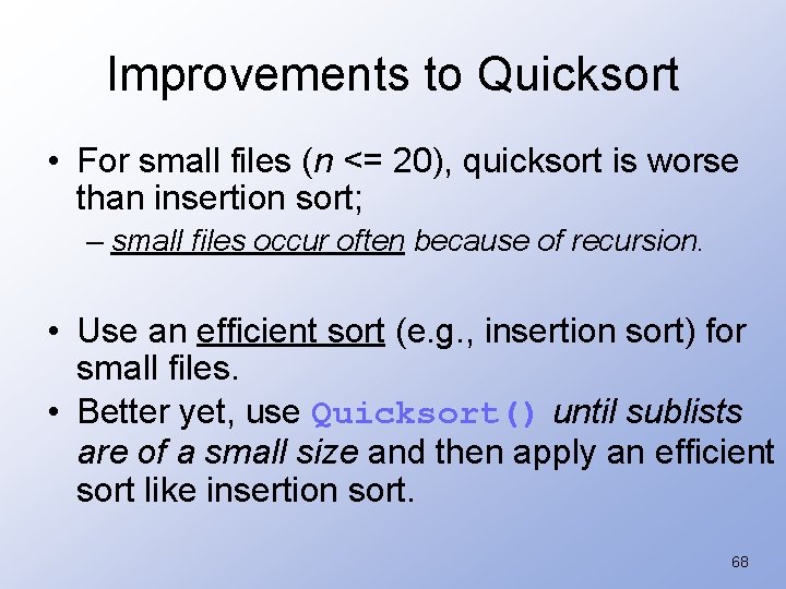
Improvements to Quicksort • For small files (n <= 20), quicksort is worse than insertion sort; – small files occur often because of recursion. • Use an efficient sort (e. g. , insertion sort) for small files. • Better yet, use Quicksort() until sublists are of a small size and then apply an efficient sort like insertion sort. 68

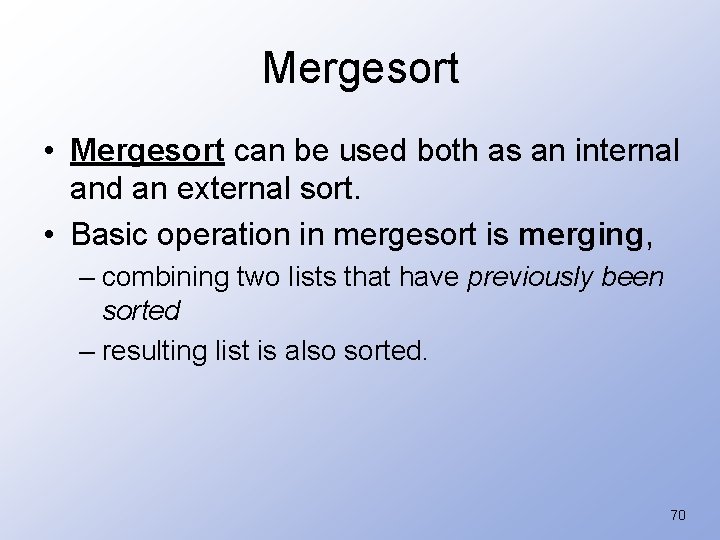
Mergesort • Sorting schemes are either … • internal -- designed for data items stored in main memory • external -- designed for data items stored in secondary memory. • Previous sorting schemes were all internal sorting algorithms: – required direct access to list elements • not possible for sequential files – made many passes through the list • not practical for files 69

Mergesort • Mergesort can be used both as an internal and an external sort. • Basic operation in mergesort is merging, – combining two lists that have previously been sorted – resulting list is also sorted. 70

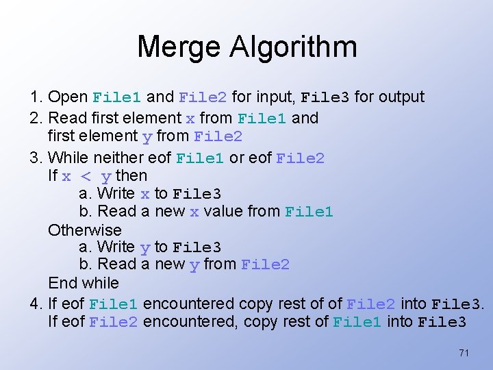
Merge Algorithm 1. Open File 1 and File 2 for input, File 3 for output 2. Read first element x from File 1 and first element y from File 2 3. While neither eof File 1 or eof File 2 If x < y then a. Write x to File 3 b. Read a new x value from File 1 Otherwise a. Write y to File 3 b. Read a new y from File 2 End while 4. If eof File 1 encountered copy rest of of File 2 into File 3. If eof File 2 encountered, copy rest of File 1 into File 3 71

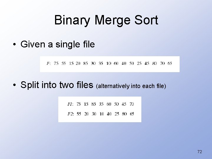
Binary Merge Sort • Given a single file • Split into two files (alternatively into each file) 72

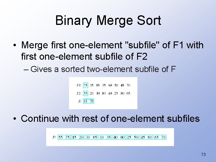
Binary Merge Sort • Merge first one-element "subfile" of F 1 with first one-element subfile of F 2 – Gives a sorted two-element subfile of F • Continue with rest of one-element subfiles 73

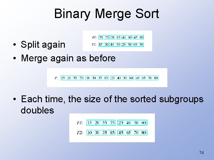
Binary Merge Sort • Split again • Merge again as before • Each time, the size of the sorted subgroups doubles 74

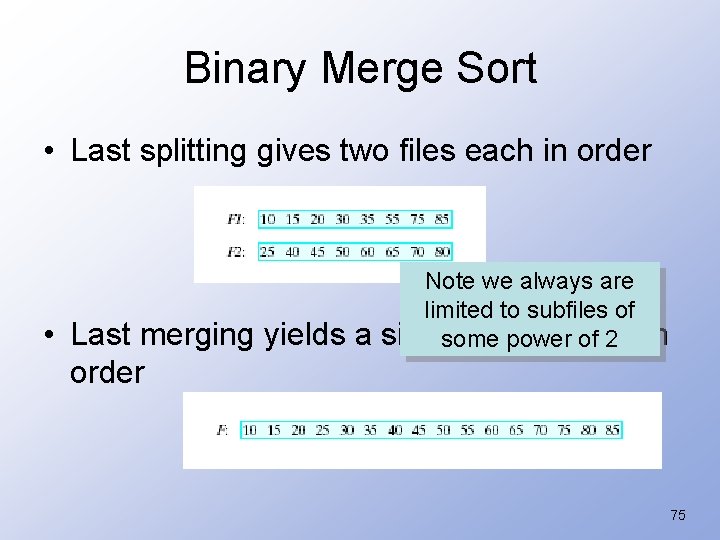
Binary Merge Sort • Last splitting gives two files each in order • Note we always are limited to subfiles of Last merging yields a single file, entirely in some power of 2 order 75

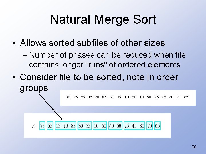
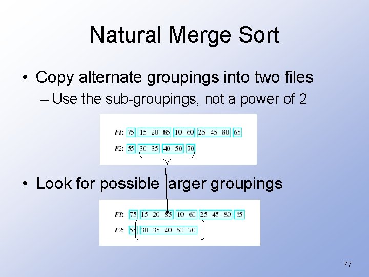
Natural Merge Sort • Allows sorted subfiles of other sizes – Number of phases can be reduced when file contains longer "runs" of ordered elements • Consider file to be sorted, note in order groups 76

Natural Merge Sort • Copy alternate groupings into two files – Use the sub-groupings, not a power of 2 • Look for possible larger groupings 77

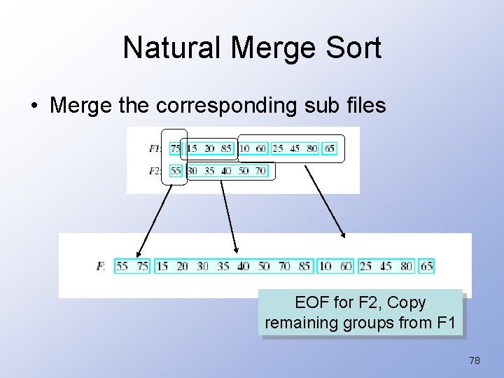
Natural Merge Sort • Merge the corresponding sub files EOF for F 2, Copy remaining groups from F 1 78

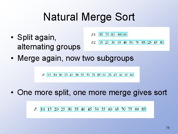
Natural Merge Sort • Split again, alternating groups • Merge again, now two subgroups • One more split, one more merge gives sort 79

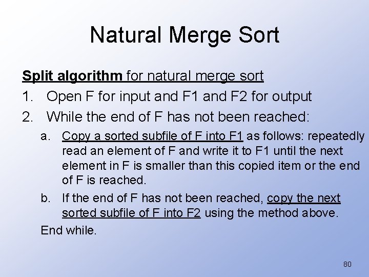
Natural Merge Sort Split algorithm for natural merge sort 1. Open F for input and F 1 and F 2 for output 2. While the end of F has not been reached: a. Copy a sorted subfile of F into F 1 as follows: repeatedly read an element of F and write it to F 1 until the next element in F is smaller than this copied item or the end of F is reached. b. If the end of F has not been reached, copy the next sorted subfile of F into F 2 using the method above. End while. 80

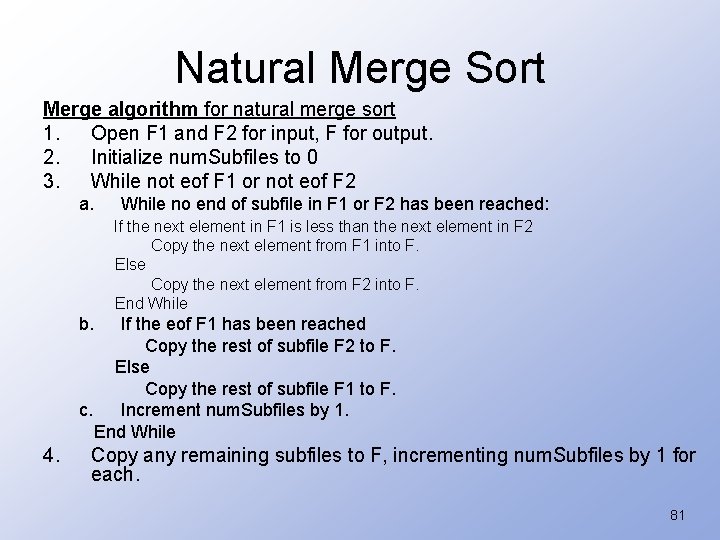
Natural Merge Sort Merge algorithm for natural merge sort 1. Open F 1 and F 2 for input, F for output. 2. Initialize num. Subfiles to 0 3. While not eof F 1 or not eof F 2 a. While no end of subfile in F 1 or F 2 has been reached: If the next element in F 1 is less than the next element in F 2 Copy the next element from F 1 into F. Else Copy the next element from F 2 into F. End While b. If the eof F 1 has been reached Copy the rest of subfile F 2 to F. Else Copy the rest of subfile F 1 to F. c. Increment num. Subfiles by 1. End While 4. Copy any remaining subfiles to F, incrementing num. Subfiles by 1 for each. 81

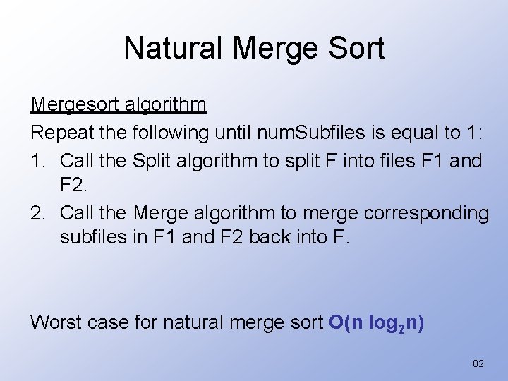
Natural Merge Sort Mergesort algorithm Repeat the following until num. Subfiles is equal to 1: 1. Call the Split algorithm to split F into files F 1 and F 2. 2. Call the Merge algorithm to merge corresponding subfiles in F 1 and F 2 back into F. Worst case for natural merge sort O(n log 2 n) 82

Natural Merge. Sort Example 83

Natural Merge. Sort Review 84

Natural Merge. Sort Review So forth and so on… 85

Natural Merge. Sort Review 86

Recursive Natural Merge. Sort 87

Recursive Natural Merge. Sort 88

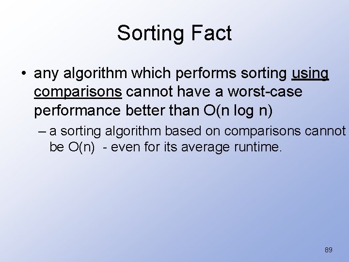
Sorting Fact • any algorithm which performs sorting using comparisons cannot have a worst-case performance better than O(n log n) – a sorting algorithm based on comparisons cannot be O(n) - even for its average runtime. 89

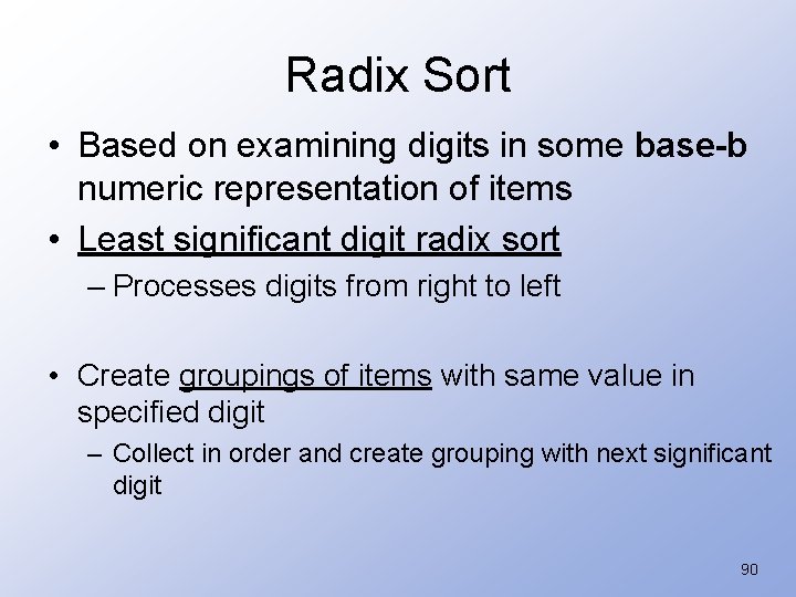
Radix Sort • Based on examining digits in some base-b numeric representation of items • Least significant digit radix sort – Processes digits from right to left • Create groupings of items with same value in specified digit – Collect in order and create grouping with next significant digit 90

Radix Sort Order ten 2 digit numbers in 10 bins from smallest number to largest number. Requires 2 calls to the sort Algorithm. Initial Sequence: Pass 0: 91 6 85 15 92 35 30 22 39 Distribute the cards into bins according to the 1's digit (100). 91

Radix Sort Final Sequence: Pass 1: 91 6 85 15 92 35 30 22 39 Take the new sequence and distribute the cards into bins determined by the 10's digit (101). 92

Sort Algorithm Analysis • Selection Sort (uses a swap) – Worst and average case O(n^2) – can be used with linked-list (doesn’t require random-access data) – Can be done in place – not at all fast for nearly sorted data 93

Sort Algorithm Analysis • Bubble Sort (uses an exchange) – Worst and average case O(n^2) – Since it is using localized exchanges - can be used with linked-list – Can be done in place – O(n^2) - even if only one item is out of place 94

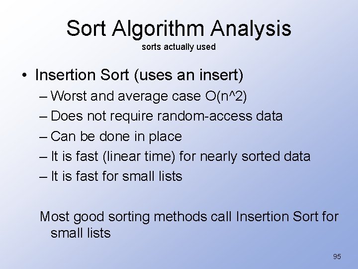
Sort Algorithm Analysis sorts actually used • Insertion Sort (uses an insert) – Worst and average case O(n^2) – Does not require random-access data – Can be done in place – It is fast (linear time) for nearly sorted data – It is fast for small lists Most good sorting methods call Insertion Sort for small lists 95

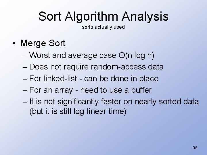
Sort Algorithm Analysis sorts actually used • Merge Sort – Worst and average case O(n log n) – Does not require random-access data – For linked-list - can be done in place – For an array - need to use a buffer – It is not significantly faster on nearly sorted data (but it is still log-linear time) 96

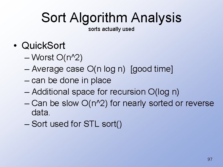
Sort Algorithm Analysis sorts actually used • Quick. Sort – Worst O(n^2) – Average case O(n log n) [good time] – can be done in place – Additional space for recursion O(log n) – Can be slow O(n^2) for nearly sorted or reverse data. – Sort used for STL sort() 97

End of sorting 98