Hough Transforms CSE 4310 Computer Vision Vassilis Athitsos

![An Example rhos = [-7, -5, -3, -1, 1, 3, 5, 7] # 8 An Example rhos = [-7, -5, -3, -1, 1, 3, 5, 7] # 8](https://slidetodoc.com/presentation_image_h2/7eea407394557e0b366935997cc28421/image-26.jpg)
![An Example rhos = [-7, -5, -3, -1, 1, 3, 5, 7] # 8 An Example rhos = [-7, -5, -3, -1, 1, 3, 5, 7] # 8](https://slidetodoc.com/presentation_image_h2/7eea407394557e0b366935997cc28421/image-27.jpg)
![An Example rhos = [-7, -5, -3, -1, 1, 3, 5, 7] # 8 An Example rhos = [-7, -5, -3, -1, 1, 3, 5, 7] # 8](https://slidetodoc.com/presentation_image_h2/7eea407394557e0b366935997cc28421/image-28.jpg)
![An Example rhos = [-7, -5, -3, -1, 1, 3, 5, 7] # 8 An Example rhos = [-7, -5, -3, -1, 1, 3, 5, 7] # 8](https://slidetodoc.com/presentation_image_h2/7eea407394557e0b366935997cc28421/image-29.jpg)
![An Example rhos = [-7, -5, -3, -1, 1, 3, 5, 7] # 8 An Example rhos = [-7, -5, -3, -1, 1, 3, 5, 7] # 8](https://slidetodoc.com/presentation_image_h2/7eea407394557e0b366935997cc28421/image-30.jpg)
![An Example rhos = [-7, -5, -3, -1, 1, 3, 5, 7] # 8 An Example rhos = [-7, -5, -3, -1, 1, 3, 5, 7] # 8](https://slidetodoc.com/presentation_image_h2/7eea407394557e0b366935997cc28421/image-31.jpg)
![An Example rhos = [-7, -5, -3, -1, 1, 3, 5, 7] # 8 An Example rhos = [-7, -5, -3, -1, 1, 3, 5, 7] # 8](https://slidetodoc.com/presentation_image_h2/7eea407394557e0b366935997cc28421/image-32.jpg)
![An Example rhos = [-7, -5, -3, -1, 1, 3, 5, 7] # 8 An Example rhos = [-7, -5, -3, -1, 1, 3, 5, 7] # 8](https://slidetodoc.com/presentation_image_h2/7eea407394557e0b366935997cc28421/image-33.jpg)
![An Example rhos = [-7, -5, -3, -1, 1, 3, 5, 7] # 8 An Example rhos = [-7, -5, -3, -1, 1, 3, 5, 7] # 8](https://slidetodoc.com/presentation_image_h2/7eea407394557e0b366935997cc28421/image-34.jpg)
![An Example rhos = [-7, -5, -3, -1, 1, 3, 5, 7] # 8 An Example rhos = [-7, -5, -3, -1, 1, 3, 5, 7] # 8](https://slidetodoc.com/presentation_image_h2/7eea407394557e0b366935997cc28421/image-35.jpg)
![An Example rhos = [-7, -5, -3, -1, 1, 3, 5, 7] # 8 An Example rhos = [-7, -5, -3, -1, 1, 3, 5, 7] # 8](https://slidetodoc.com/presentation_image_h2/7eea407394557e0b366935997cc28421/image-36.jpg)
![An Example rhos = [-7, -5, -3, -1, 1, 3, 5, 7] # 8 An Example rhos = [-7, -5, -3, -1, 1, 3, 5, 7] # 8](https://slidetodoc.com/presentation_image_h2/7eea407394557e0b366935997cc28421/image-37.jpg)
![An Example rhos = [-7, -5, -3, -1, 1, 3, 5, 7] # 8 An Example rhos = [-7, -5, -3, -1, 1, 3, 5, 7] # 8](https://slidetodoc.com/presentation_image_h2/7eea407394557e0b366935997cc28421/image-38.jpg)
![An Example rhos = [-7, -5, -3, -1, 1, 3, 5, 7] # 8 An Example rhos = [-7, -5, -3, -1, 1, 3, 5, 7] # 8](https://slidetodoc.com/presentation_image_h2/7eea407394557e0b366935997cc28421/image-39.jpg)
![An Example rhos = [-7, -5, -3, -1, 1, 3, 5, 7] # 8 An Example rhos = [-7, -5, -3, -1, 1, 3, 5, 7] # 8](https://slidetodoc.com/presentation_image_h2/7eea407394557e0b366935997cc28421/image-40.jpg)
![An Example rhos = [-7, -5, -3, -1, 1, 3, 5, 7] # 8 An Example rhos = [-7, -5, -3, -1, 1, 3, 5, 7] # 8](https://slidetodoc.com/presentation_image_h2/7eea407394557e0b366935997cc28421/image-41.jpg)
![An Example rhos = [-7, -5, -3, -1, 1, 3, 5, 7] # 8 An Example rhos = [-7, -5, -3, -1, 1, 3, 5, 7] # 8](https://slidetodoc.com/presentation_image_h2/7eea407394557e0b366935997cc28421/image-42.jpg)

- Slides: 82

Hough Transforms CSE 4310 – Computer Vision Vassilis Athitsos Computer Science and Engineering Department University of Texas at Arlington 1

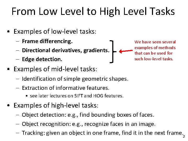
From Low Level to High Level Tasks • Examples of low-level tasks: – Frame differencing. – Directional derivatives, gradients. – Edge detection. We have seen several examples of methods that can be used for such low-level tasks. • Examples of mid-level tasks: – Identification of simple geometric shapes. – Extraction of informative features. • see later lectures on SIFT and HOG features. • Examples of high-level tasks: – Object detection: e. g. , find bounding boxes of faces. – Object recognition: e. g. , recognize faces in an image. – Tracking: given an object in one frame, find it in the next frame. 2

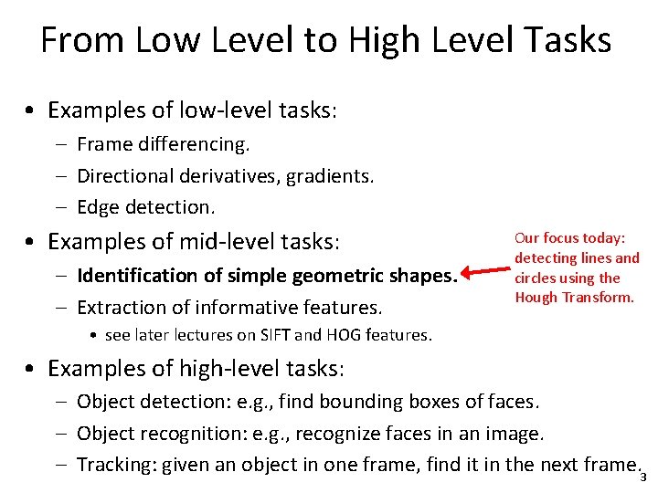
From Low Level to High Level Tasks • Examples of low-level tasks: – Frame differencing. – Directional derivatives, gradients. – Edge detection. • Examples of mid-level tasks: – Identification of simple geometric shapes. – Extraction of informative features. Our focus today: detecting lines and circles using the Hough Transform. • see later lectures on SIFT and HOG features. • Examples of high-level tasks: – Object detection: e. g. , find bounding boxes of faces. – Object recognition: e. g. , recognize faces in an image. – Tracking: given an object in one frame, find it in the next frame. 3

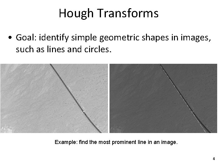
Hough Transforms • Goal: identify simple geometric shapes in images, such as lines and circles. Example: find the most prominent line in an image. 4

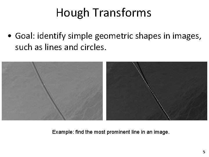
Hough Transforms • Goal: identify simple geometric shapes in images, such as lines and circles. Example: find the most prominent line in an image. 5

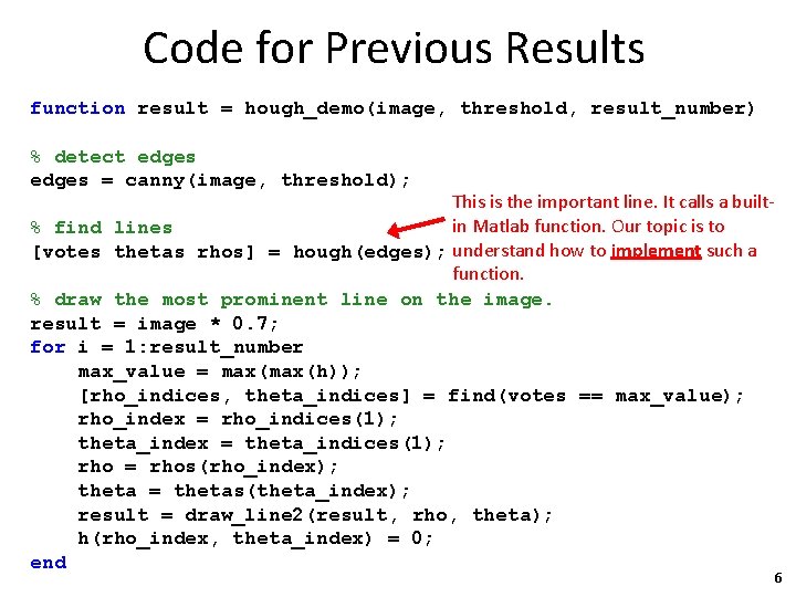
Code for Previous Results function result = hough_demo(image, threshold, result_number) % detect edges = canny(image, threshold); This is the important line. It calls a builtin Matlab function. Our topic is to % find lines [votes thetas rhos] = hough(edges); understand how to implement such a function. % draw the most prominent line on the image. result = image * 0. 7; for i = 1: result_number max_value = max(h)); [rho_indices, theta_indices] = find(votes == max_value); rho_index = rho_indices(1); theta_index = theta_indices(1); rho = rhos(rho_index); theta = thetas(theta_index); result = draw_line 2(result, rho, theta); h(rho_index, theta_index) = 0; end 6

What is a Straight Line? 7

What is a Straight Line? • It is infinite. • It is the shortest path that connects two points in space (or in a 2 D image, in our case). • It is defined in multiple ways (see next slides). 8

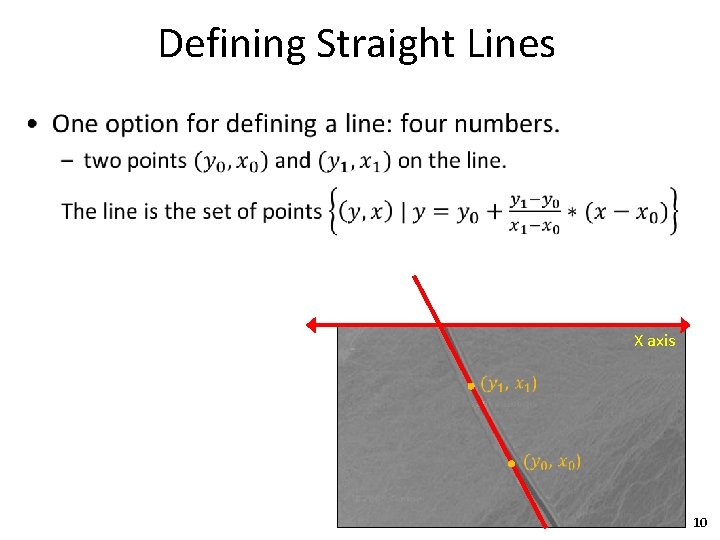
Defining Straight Lines • How many parameters do we need to define a line on an image? 9

Defining Straight Lines • X axis 10

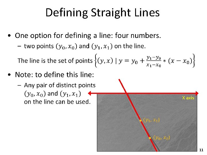
Defining Straight Lines • X axis 11

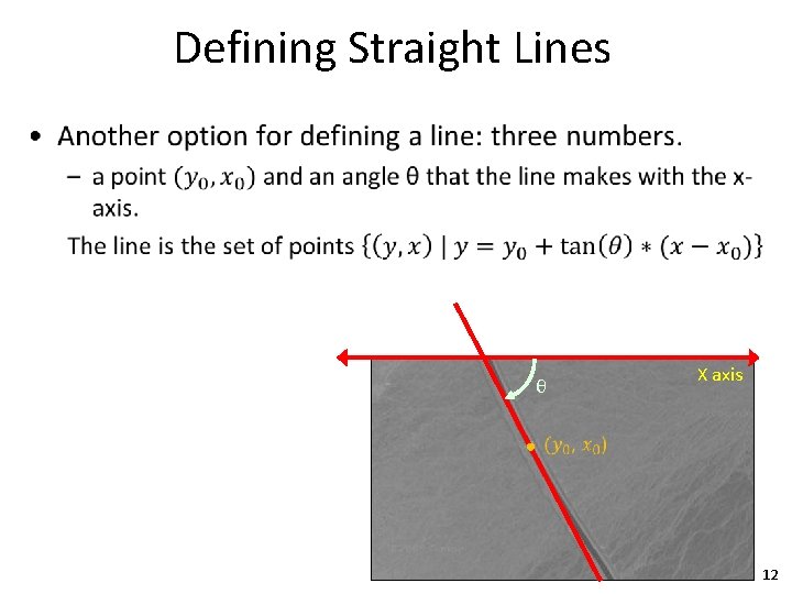
Defining Straight Lines • θ X axis 12

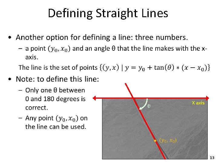
Defining Straight Lines • θ X axis 13

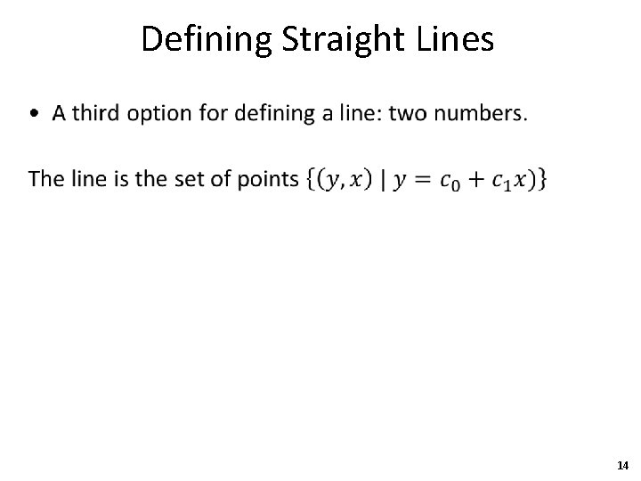
Defining Straight Lines • 14

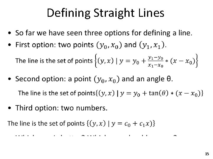
Defining Straight Lines • 15

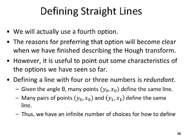
Defining Straight Lines • 16

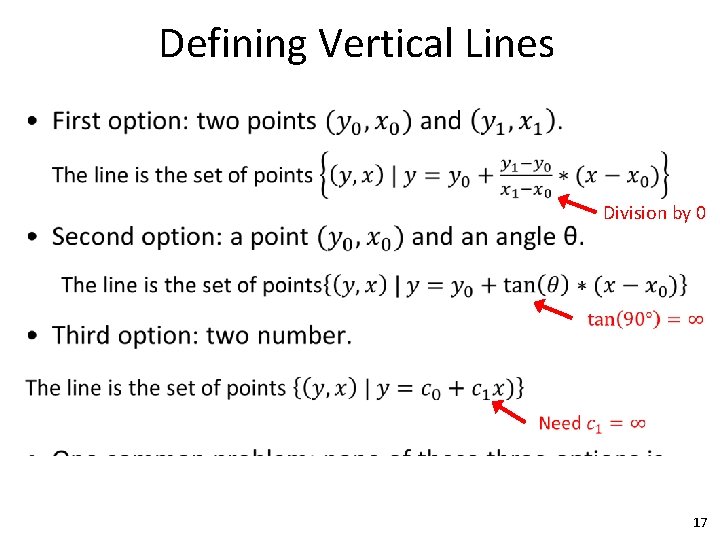
Defining Vertical Lines • Division by 0 17

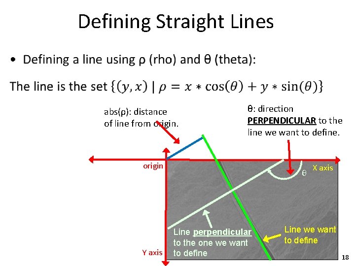
Defining Straight Lines • abs(ρ): distance of line from origin. θ: direction PERPENDICULAR to the line we want to define. origin Y axis θ Line perpendicular to the one we want to define X axis Line we want to define 18

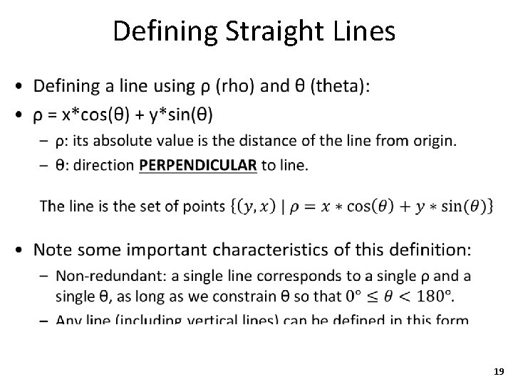
Defining Straight Lines • 19

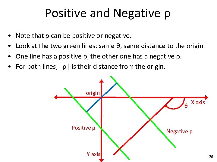
Positive and Negative ρ • • Note that ρ can be positive or negative. Look at the two green lines: same θ, same distance to the origin. One line has a positive ρ, the other one has a negative ρ. For both lines, |ρ| is their distance from the origin θ Positive ρ Y axis X axis Negative ρ 20

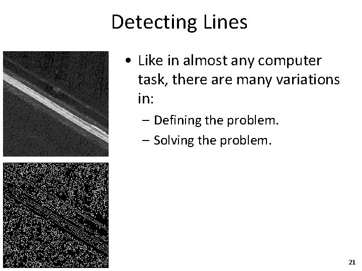
Detecting Lines • Like in almost any computer task, there are many variations in: – Defining the problem. – Solving the problem. 21

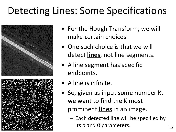
Detecting Lines: Some Specifications • For the Hough Transform, we will make certain choices. • One such choice is that we will detect lines, not line segments. • A line segment has specific endpoints. • A line is infinite. • So, given as input some number K, we want to find the K most prominent lines in an image. – Each detected line will be specified by its ρ and θ parameters. 22

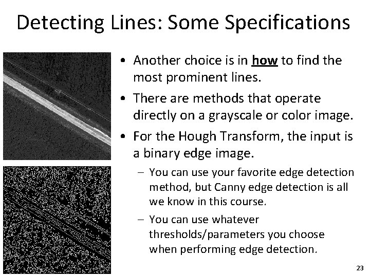
Detecting Lines: Some Specifications • Another choice is in how to find the most prominent lines. • There are methods that operate directly on a grayscale or color image. • For the Hough Transform, the input is a binary edge image. – You can use your favorite edge detection method, but Canny edge detection is all we know in this course. – You can use whatever thresholds/parameters you choose when performing edge detection. 23

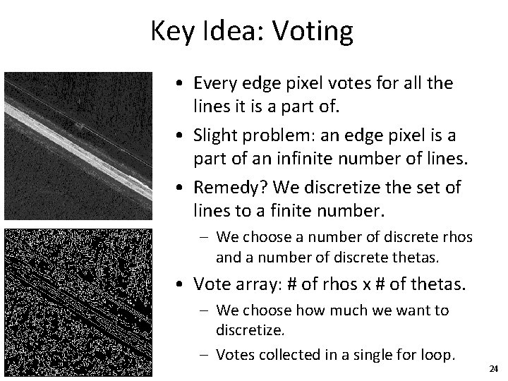
Key Idea: Voting • Every edge pixel votes for all the lines it is a part of. • Slight problem: an edge pixel is a part of an infinite number of lines. • Remedy? We discretize the set of lines to a finite number. – We choose a number of discrete rhos and a number of discrete thetas. • Vote array: # of rhos x # of thetas. – We choose how much we want to discretize. – Votes collected in a single for loop. 24

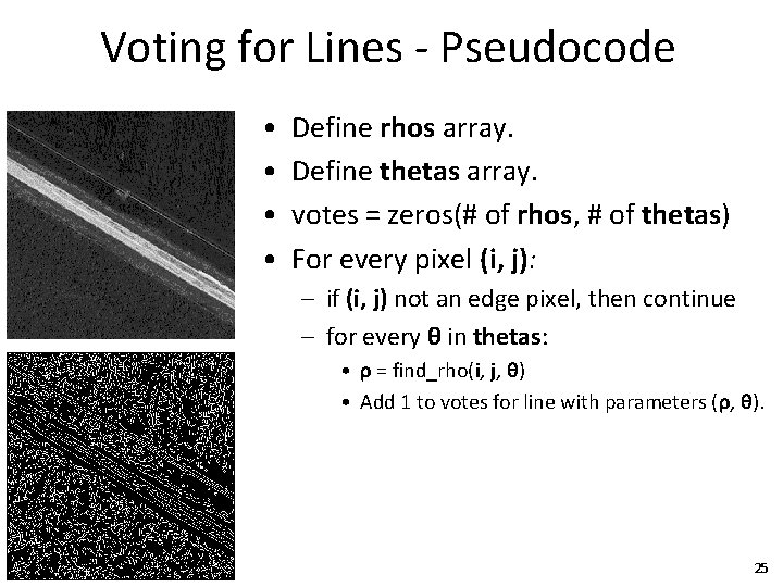
Voting for Lines - Pseudocode • • Define rhos array. Define thetas array. votes = zeros(# of rhos, # of thetas) For every pixel (i, j): – if (i, j) not an edge pixel, then continue – for every θ in thetas: • ρ = find_rho(i, j, θ) • Add 1 to votes for line with parameters (ρ, θ). 25
![An Example rhos 7 5 3 1 1 3 5 7 8 An Example rhos = [-7, -5, -3, -1, 1, 3, 5, 7] # 8](https://slidetodoc.com/presentation_image_h2/7eea407394557e0b366935997cc28421/image-26.jpg)
An Example rhos = [-7, -5, -3, -1, 1, 3, 5, 7] # 8 values thetas = [-90, -75, -60, -45, -30, -15, 0, 15, 30, 45, 60, 75] # 12 values Do we have any other options for rhos and thetas? Size of voting array: ? ? ? origin Y axis X axis Input: 11 x 11 binary edge image. 26
![An Example rhos 7 5 3 1 1 3 5 7 8 An Example rhos = [-7, -5, -3, -1, 1, 3, 5, 7] # 8](https://slidetodoc.com/presentation_image_h2/7eea407394557e0b366935997cc28421/image-27.jpg)
An Example rhos = [-7, -5, -3, -1, 1, 3, 5, 7] # 8 values thetas = [-90, -75, -60, -45, -30, -15, 0, 15, 30, 45, 60, 75] # 12 values # Note: the above choices are arbitrary choices for discretizing ρ and θ values. Size of voting array: 8 x 12 - votes = zeros(8, 12) - For each pixel: - If it is an edge pixel: - For each θ in thetas: - find the corresponding ρ. - Add a vote to the position in the voting array for that ρ and θ. origin Y axis X axis Input: 11 x 11 binary edge image. 27
![An Example rhos 7 5 3 1 1 3 5 7 8 An Example rhos = [-7, -5, -3, -1, 1, 3, 5, 7] # 8](https://slidetodoc.com/presentation_image_h2/7eea407394557e0b366935997cc28421/image-28.jpg)
An Example rhos = [-7, -5, -3, -1, 1, 3, 5, 7] # 8 values thetas = [-90, -75, -60, -45, -30, -15, 0, 15, 30, 45, 60, 75] # 12 values # Note: the above choices are arbitrary choices for discretizing ρ and θ values. - Suppose we get to pixel (2, 2). For each θ in thetas: - what do we do? X axis origin Y axis Input: 11 x 11 binary edge image. 28
![An Example rhos 7 5 3 1 1 3 5 7 8 An Example rhos = [-7, -5, -3, -1, 1, 3, 5, 7] # 8](https://slidetodoc.com/presentation_image_h2/7eea407394557e0b366935997cc28421/image-29.jpg)
An Example rhos = [-7, -5, -3, -1, 1, 3, 5, 7] # 8 values thetas = [-90, -75, -60, -45, -30, -15, 0, 15, 30, 45, 60, 75] # 12 values # Note: the above choices are arbitrary choices for discretizing ρ and θ values. - Suppose we get to pixel (2, 2). For each θ in thetas: - Find the corresponding ρ. - Add a vote to the position in the voting array for that ρ and θ. X axis origin Y axis Input: 11 x 11 binary edge image. 29
![An Example rhos 7 5 3 1 1 3 5 7 8 An Example rhos = [-7, -5, -3, -1, 1, 3, 5, 7] # 8](https://slidetodoc.com/presentation_image_h2/7eea407394557e0b366935997cc28421/image-30.jpg)
An Example rhos = [-7, -5, -3, -1, 1, 3, 5, 7] # 8 values thetas = [-90, -75, -60, -45, -30, -15, 0, 15, 30, 45, 60, 75] # 12 values # Note: the above choices are arbitrary choices for discretizing ρ and θ values. - Start with θ = -90 degrees. Remember, θ is the direction perpendicular to the line. - So, the line itself has orientation 0 degrees. - ρ = ? ? ? X axis origin Y axis Input: 11 x 11 binary edge image. 30
![An Example rhos 7 5 3 1 1 3 5 7 8 An Example rhos = [-7, -5, -3, -1, 1, 3, 5, 7] # 8](https://slidetodoc.com/presentation_image_h2/7eea407394557e0b366935997cc28421/image-31.jpg)
An Example rhos = [-7, -5, -3, -1, 1, 3, 5, 7] # 8 values thetas = [-90, -75, -60, -45, -30, -15, 0, 15, 30, 45, 60, 75] # 12 values # Note: the above choices are arbitrary choices for discretizing ρ and θ values. - Start with θ = -90 degrees. Remember, θ is the direction perpendicular to the line. - So, the line itself has orientation 0 degrees. - ρ = x cos(θ) + y sin(θ) = 2*0+2*(-1) = -2. X axis origin What do we vote for? Y axis Input: 11 x 11 binary edge image. 31
![An Example rhos 7 5 3 1 1 3 5 7 8 An Example rhos = [-7, -5, -3, -1, 1, 3, 5, 7] # 8](https://slidetodoc.com/presentation_image_h2/7eea407394557e0b366935997cc28421/image-32.jpg)
An Example rhos = [-7, -5, -3, -1, 1, 3, 5, 7] # 8 values thetas = [-90, -75, -60, -45, -30, -15, 0, 15, 30, 45, 60, 75] # 12 values # Note: the above choices are arbitrary choices for discretizing ρ and θ values. - Start with θ = -90 degrees. Remember, θ is the direction perpendicular to the line. - So, the line itself has orientation 0 degrees. - ρ = x cos(θ) + y sin(θ) = 2*0+2*(-1) = -2. What do we vote for? - The closest values to -2 in rhos are -3 and -1 (-2 is half way between). - Ties like this are rare, but they can happen. X axis origin Y axis Input: 11 x 11 binary edge image. 32
![An Example rhos 7 5 3 1 1 3 5 7 8 An Example rhos = [-7, -5, -3, -1, 1, 3, 5, 7] # 8](https://slidetodoc.com/presentation_image_h2/7eea407394557e0b366935997cc28421/image-33.jpg)
An Example rhos = [-7, -5, -3, -1, 1, 3, 5, 7] # 8 values thetas = [-90, -75, -60, -45, -30, -15, 0, 15, 30, 45, 60, 75] # 12 values # Note: the above choices are arbitrary choices for discretizing ρ and θ values. - Start with θ = -90 degrees. Remember, θ is the direction perpendicular to the line. - So, the line itself has orientation 0 degrees. - ρ = x cos(θ) + y sin(θ) = 2*0+2*(-1) = -2. What do we vote for? - The closest values to -2 in rhos are -3 and -1 (-2 is half way between). - So, we can split our vote between (ρ=-3, θ=-90) and (ρ=-1, θ=-90) X axis origin Y axis Input: 11 x 11 binary edge image. 33
![An Example rhos 7 5 3 1 1 3 5 7 8 An Example rhos = [-7, -5, -3, -1, 1, 3, 5, 7] # 8](https://slidetodoc.com/presentation_image_h2/7eea407394557e0b366935997cc28421/image-34.jpg)
An Example rhos = [-7, -5, -3, -1, 1, 3, 5, 7] # 8 values thetas = [-90, -75, -60, -45, -30, -15, 0, 15, 30, 45, 60, 75] # 12 values # Note: the above choices are arbitrary choices for discretizing ρ and θ values. We want to give 0. 5 vote to each of (ρ=-3, θ=-90) and (ρ=-1, θ=-90). X axis origin Remember, we have a voting array called votes, of size 8 x 12. Which position in votes corresponds to (ρ=-3, θ=-90)? Y axis Input: 11 x 11 binary edge image. 34
![An Example rhos 7 5 3 1 1 3 5 7 8 An Example rhos = [-7, -5, -3, -1, 1, 3, 5, 7] # 8](https://slidetodoc.com/presentation_image_h2/7eea407394557e0b366935997cc28421/image-35.jpg)
An Example rhos = [-7, -5, -3, -1, 1, 3, 5, 7] # 8 values thetas = [-90, -75, -60, -45, -30, -15, 0, 15, 30, 45, 60, 75] # 12 values # Note: the above choices are arbitrary choices for discretizing ρ and θ values. We want to give 0. 5 vote to each of (ρ=-3, θ=-90) and (ρ=-1, θ=-90). X axis origin Remember, we have a voting array called votes, of size 8 x 12. Which position in votes corresponds to (ρ=-3, θ=-90)? -3 is at position 3 in rhos. -90 is at position 1 in thetas. Therefore, we add 0. 5 to votes(3, 1). Y axis Input: 11 x 11 binary edge image. 35
![An Example rhos 7 5 3 1 1 3 5 7 8 An Example rhos = [-7, -5, -3, -1, 1, 3, 5, 7] # 8](https://slidetodoc.com/presentation_image_h2/7eea407394557e0b366935997cc28421/image-36.jpg)
An Example rhos = [-7, -5, -3, -1, 1, 3, 5, 7] # 8 values thetas = [-90, -75, -60, -45, -30, -15, 0, 15, 30, 45, 60, 75] # 12 values # Note: the above choices are arbitrary choices for discretizing ρ and θ values. We want to give 0. 5 vote to each of (ρ=-3, θ=-90) and (ρ=-1, θ=-90). X axis origin Remember, we have a voting array called votes, of size 8 x 12. Which position in votes corresponds to (ρ=-1, θ=-90)? -1 is at position 4 in rhos. -90 is at position 1 in thetas. Therefore, we add 0. 5 to votes(4, 1). Y axis Input: 11 x 11 binary edge image. 36
![An Example rhos 7 5 3 1 1 3 5 7 8 An Example rhos = [-7, -5, -3, -1, 1, 3, 5, 7] # 8](https://slidetodoc.com/presentation_image_h2/7eea407394557e0b366935997cc28421/image-37.jpg)
An Example rhos = [-7, -5, -3, -1, 1, 3, 5, 7] # 8 values thetas = [-90, -75, -60, -45, -30, -15, 0, 15, 30, 45, 60, 75] # 12 values # Note: the above choices are arbitrary choices for discretizing ρ and θ values. What do we do next? X axis origin Y axis Input: 11 x 11 binary edge image. 37
![An Example rhos 7 5 3 1 1 3 5 7 8 An Example rhos = [-7, -5, -3, -1, 1, 3, 5, 7] # 8](https://slidetodoc.com/presentation_image_h2/7eea407394557e0b366935997cc28421/image-38.jpg)
An Example rhos = [-7, -5, -3, -1, 1, 3, 5, 7] # 8 values thetas = [-90, -75, -60, -45, -30, -15, 0, 15, 30, 45, 60, 75] # 12 values # Note: the above choices are arbitrary choices for discretizing ρ and θ values. - Next θ = -75 degrees. Remember, θ is the direction perpendicular to the line. - So, the line itself has orientation 15 degrees. - ρ = x cos(θ) + y sin(θ) = 2*cos(-75)+2*sin(-75) = -1. 414. X axis origin What do we vote for? Y axis Input: 11 x 11 binary edge image. 38
![An Example rhos 7 5 3 1 1 3 5 7 8 An Example rhos = [-7, -5, -3, -1, 1, 3, 5, 7] # 8](https://slidetodoc.com/presentation_image_h2/7eea407394557e0b366935997cc28421/image-39.jpg)
An Example rhos = [-7, -5, -3, -1, 1, 3, 5, 7] # 8 values thetas = [-90, -75, -60, -45, -30, -15, 0, 15, 30, 45, 60, 75] # 12 values # Note: the above choices are arbitrary choices for discretizing ρ and θ values. - Next θ = -75 degrees. Remember, θ is the direction perpendicular to the line. - So, the line itself has orientation 15 degrees. - ρ = x cos(θ) + y sin(θ) = 2*cos(-75)+2*sin(-75) = -1. 414. What do we vote for? - The closest value to -1. 414 in rhos is -1. - So, we vote for ρ=-1, θ=-75. X axis origin Y axis Input: 11 x 11 binary edge image. 39
![An Example rhos 7 5 3 1 1 3 5 7 8 An Example rhos = [-7, -5, -3, -1, 1, 3, 5, 7] # 8](https://slidetodoc.com/presentation_image_h2/7eea407394557e0b366935997cc28421/image-40.jpg)
An Example rhos = [-7, -5, -3, -1, 1, 3, 5, 7] # 8 values thetas = [-90, -75, -60, -45, -30, -15, 0, 15, 30, 45, 60, 75] # 12 values # Note: the above choices are arbitrary choices for discretizing ρ and θ values. We want to vote for (ρ=-1, θ=-75). Remember, we have a voting array called votes, of size 8 x 12. X axis origin Which position in votes corresponds to (ρ=-1, θ=-75)? -1 is at position 4 in rhos. -75 is at position 2 in thetas. Therefore, we add 1 to votes(4, 2). Y axis Input: 11 x 11 binary edge image. 40
![An Example rhos 7 5 3 1 1 3 5 7 8 An Example rhos = [-7, -5, -3, -1, 1, 3, 5, 7] # 8](https://slidetodoc.com/presentation_image_h2/7eea407394557e0b366935997cc28421/image-41.jpg)
An Example rhos = [-7, -5, -3, -1, 1, 3, 5, 7] # 8 values thetas = [-90, -75, -60, -45, -30, -15, 0, 15, 30, 45, 60, 75] # 12 values # Note: the above choices are arbitrary choices for discretizing ρ and θ values. What do we do next? X axis origin Y axis Input: 11 x 11 binary edge image. 41
![An Example rhos 7 5 3 1 1 3 5 7 8 An Example rhos = [-7, -5, -3, -1, 1, 3, 5, 7] # 8](https://slidetodoc.com/presentation_image_h2/7eea407394557e0b366935997cc28421/image-42.jpg)
An Example rhos = [-7, -5, -3, -1, 1, 3, 5, 7] # 8 values thetas = [-90, -75, -60, -45, -30, -15, 0, 15, 30, 45, 60, 75] # 12 values # Note: the above choices are arbitrary choices for discretizing ρ and θ values. - - To finish processing pixel (2, 2), we continue doing the same thing for the remaining values in thetas: For each θ in those values, we find the corresponding ρ, and we add one vote for the line with parameters (ρ, θ). After we are done with pixel (2, 2), we continue processing the rest of the edge pixels the same way. X axis origin Y axis Input: 11 x 11 binary edge image. 42

Hough Transform for Lines • The method we have just described is called Hough Transform for lines. • The Hough transform for lines simply computes the votes for all lines. • There also more complicated Hough Transforms for circles and other shapes. 43

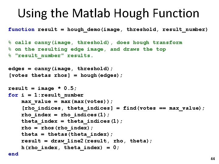
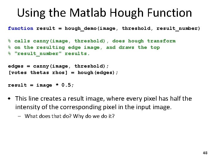
Using the Matlab Hough Function function result = hough_demo(image, threshold, result_number) % calls canny(image, threshold), does hough transform % on the resulting edge image, and draws the top % "result_number" results. edges = canny(image, threshold); [votes thetas rhos] = hough(edges); result = image * 0. 5; for i = 1: result_number max_value = max(votes)); [rho_indices, theta_indices] = find(votes == max_value); rho_index = rho_indices(1); theta_index = theta_indices(1); rho = rhos(rho_index); theta = thetas(theta_index); result = draw_line 2(result, rho, theta); h(rho_index, theta_index) = 0; end 44

Using the Matlab Hough Function function result = hough_demo(image, threshold, result_number) % calls canny(image, threshold), does hough transform % on the resulting edge image, and draws the top % "result_number" results. edges = canny(image, threshold); • For the canny function implementation, see code posted on course website. 45

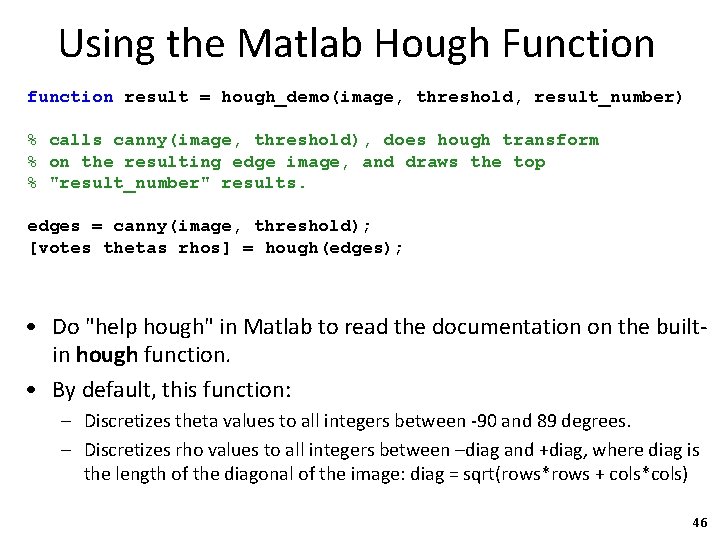
Using the Matlab Hough Function function result = hough_demo(image, threshold, result_number) % calls canny(image, threshold), does hough transform % on the resulting edge image, and draws the top % "result_number" results. edges = canny(image, threshold); [votes thetas rhos] = hough(edges); • Do "help hough" in Matlab to read the documentation on the builtin hough function. • By default, this function: – Discretizes theta values to all integers between -90 and 89 degrees. – Discretizes rho values to all integers between –diag and +diag, where diag is the length of the diagonal of the image: diag = sqrt(rows*rows + cols*cols) 46

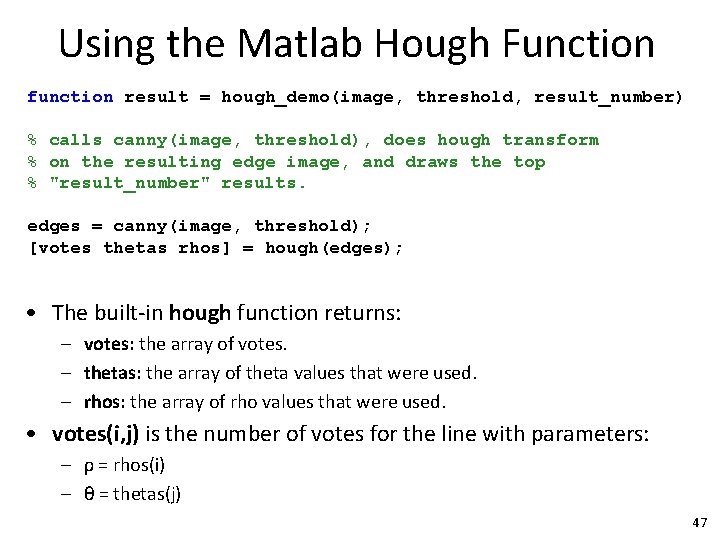
Using the Matlab Hough Function function result = hough_demo(image, threshold, result_number) % calls canny(image, threshold), does hough transform % on the resulting edge image, and draws the top % "result_number" results. edges = canny(image, threshold); [votes thetas rhos] = hough(edges); • The built-in hough function returns: – votes: the array of votes. – thetas: the array of theta values that were used. – rhos: the array of rho values that were used. • votes(i, j) is the number of votes for the line with parameters: – ρ = rhos(i) – θ = thetas(j) 47

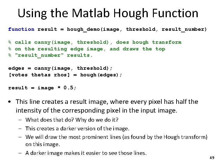
Using the Matlab Hough Function function result = hough_demo(image, threshold, result_number) % calls canny(image, threshold), does hough transform % on the resulting edge image, and draws the top % "result_number" results. edges = canny(image, threshold); [votes thetas rhos] = hough(edges); result = image * 0. 5; • This line creates a result image, where every pixel has half the intensity of the corresponding pixel in the input image. – What does that do? Why do we do it? 48

Using the Matlab Hough Function function result = hough_demo(image, threshold, result_number) % calls canny(image, threshold), does hough transform % on the resulting edge image, and draws the top % "result_number" results. edges = canny(image, threshold); [votes thetas rhos] = hough(edges); result = image * 0. 5; • This line creates a result image, where every pixel has half the intensity of the corresponding pixel in the input image. – What does that do? Why do we do it? – This creates a darker version of the image. – We will draw the most prominent lines (as found by the Hough transform) on this image. – A darker image makes it easier to see those lines. 49

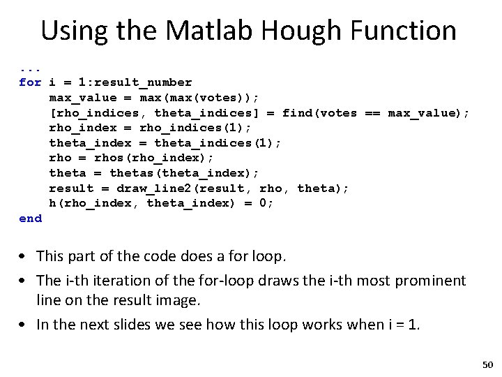
Using the Matlab Hough Function. . . for i = 1: result_number max_value = max(votes)); [rho_indices, theta_indices] = find(votes == max_value); rho_index = rho_indices(1); theta_index = theta_indices(1); rho = rhos(rho_index); theta = thetas(theta_index); result = draw_line 2(result, rho, theta); h(rho_index, theta_index) = 0; end • This part of the code does a for loop. • The i-th iteration of the for-loop draws the i-th most prominent line on the result image. • In the next slides we see how this loop works when i = 1. 50

Using the Matlab Hough Function. . . for i = 1: result_number max_value = max(votes)); . . . • We find the highest number of votes received by any of the lines. 51

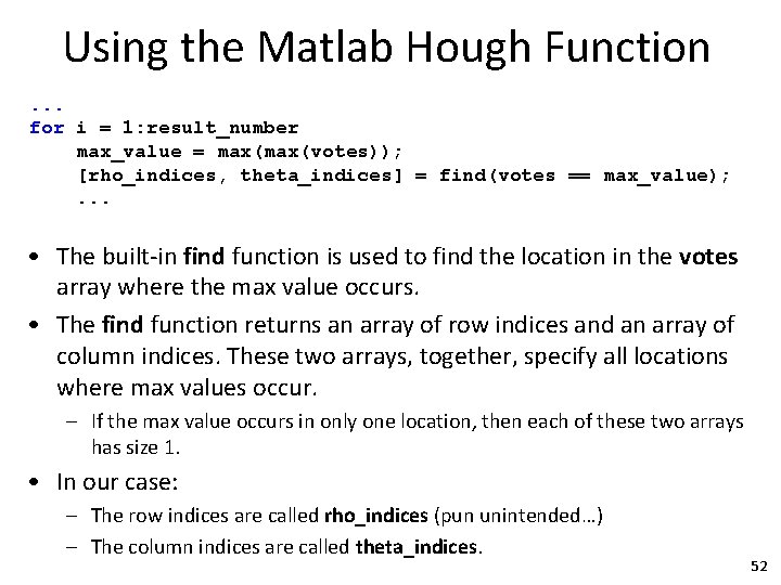
Using the Matlab Hough Function. . . for i = 1: result_number max_value = max(votes)); [rho_indices, theta_indices] = find(votes == max_value); . . . • The built-in find function is used to find the location in the votes array where the max value occurs. • The find function returns an array of row indices and an array of column indices. These two arrays, together, specify all locations where max values occur. – If the max value occurs in only one location, then each of these two arrays has size 1. • In our case: – The row indices are called rho_indices (pun unintended…) – The column indices are called theta_indices. 52

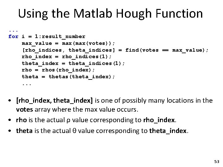
Using the Matlab Hough Function. . . for i = 1: result_number max_value = max(votes)); [rho_indices, theta_indices] = find(votes == max_value); rho_index = rho_indices(1); theta_index = theta_indices(1); rho = rhos(rho_index); theta = thetas(theta_index); . . . • [rho_index, theta_index] is one of possibly many locations in the votes array where the max value occurs. • rho is the actual ρ value corresponding to rho_index. • theta is the actual θ value corresponding to theta_index. 53

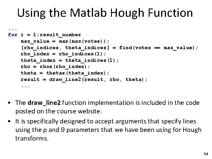
Using the Matlab Hough Function. . . for i = 1: result_number max_value = max(votes)); [rho_indices, theta_indices] = find(votes == max_value); rho_index = rho_indices(1); theta_index = theta_indices(1); rho = rhos(rho_index); theta = thetas(theta_index); result = draw_line 2(result, rho, theta); . . . • The draw_line 2 function implementation is included in the code posted on the course website. • It is specifically designed to accept arguments that specify lines using the ρ and θ parameters that we have been using for Hough transforms. 54

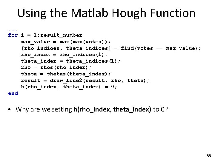
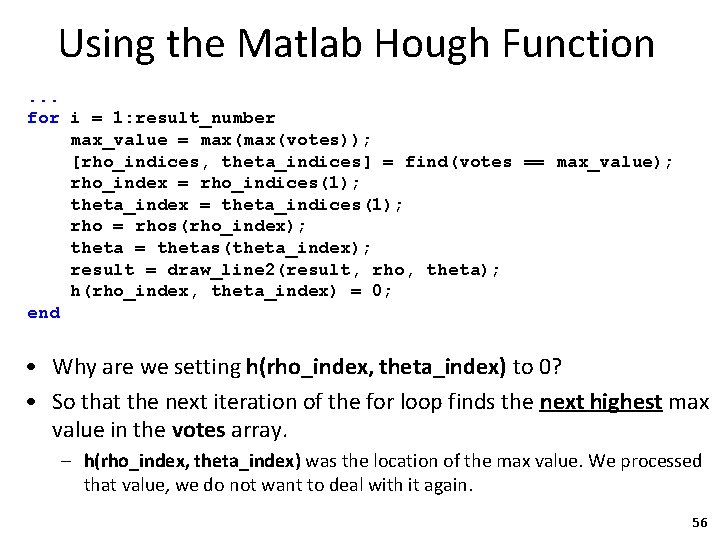
Using the Matlab Hough Function. . . for i = 1: result_number max_value = max(votes)); [rho_indices, theta_indices] = find(votes == max_value); rho_index = rho_indices(1); theta_index = theta_indices(1); rho = rhos(rho_index); theta = thetas(theta_index); result = draw_line 2(result, rho, theta); h(rho_index, theta_index) = 0; end • Why are we setting h(rho_index, theta_index) to 0? 55

Using the Matlab Hough Function. . . for i = 1: result_number max_value = max(votes)); [rho_indices, theta_indices] = find(votes == max_value); rho_index = rho_indices(1); theta_index = theta_indices(1); rho = rhos(rho_index); theta = thetas(theta_index); result = draw_line 2(result, rho, theta); h(rho_index, theta_index) = 0; end • Why are we setting h(rho_index, theta_index) to 0? • So that the next iteration of the for loop finds the next highest max value in the votes array. – h(rho_index, theta_index) was the location of the max value. We processed that value, we do not want to deal with it again. 56

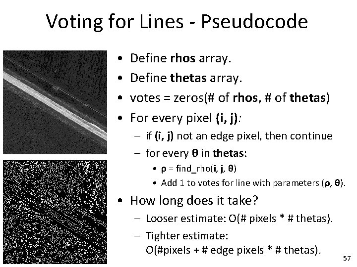
Voting for Lines - Pseudocode • • Define rhos array. Define thetas array. votes = zeros(# of rhos, # of thetas) For every pixel (i, j): – if (i, j) not an edge pixel, then continue – for every θ in thetas: • ρ = find_rho(i, j, θ) • Add 1 to votes for line with parameters (ρ, θ). • How long does it take? – Looser estimate: O(# pixels * # thetas). – Tighter estimate: O(#pixels + # edge pixels * # thetas). 57

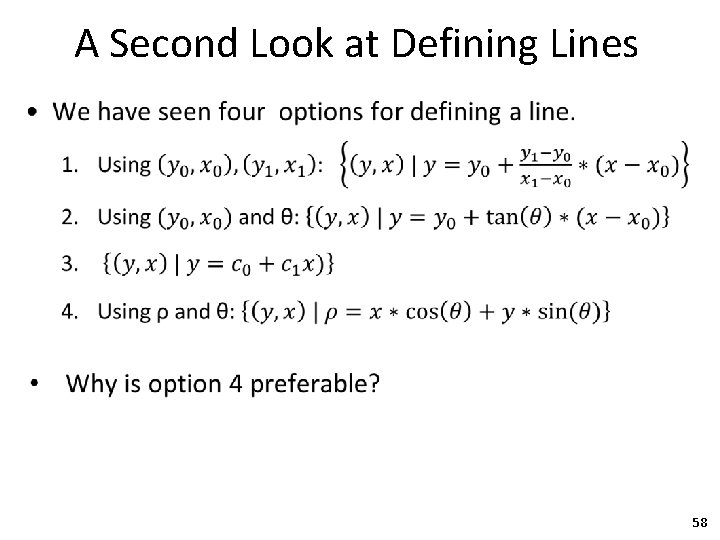
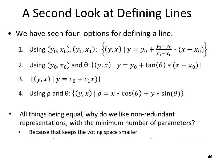
A Second Look at Defining Lines • 58

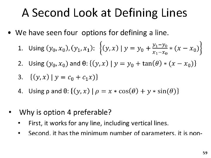
A Second Look at Defining Lines • 59

A Second Look at Defining Lines • 60

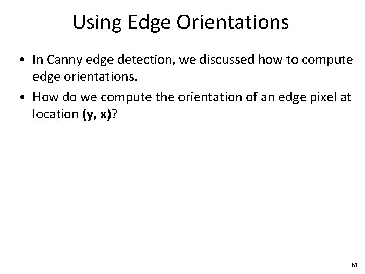
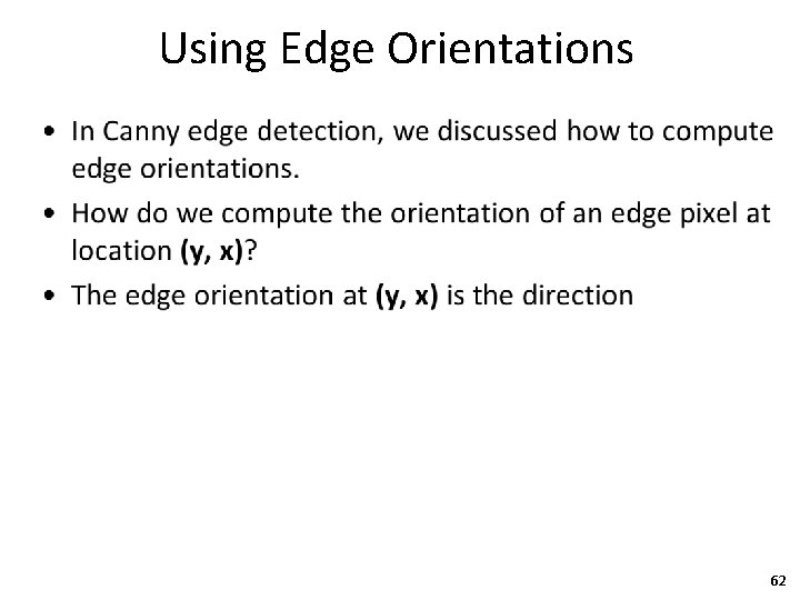
Using Edge Orientations • In Canny edge detection, we discussed how to compute edge orientations. • How do we compute the orientation of an edge pixel at location (y, x)? 61

Using Edge Orientations • 62

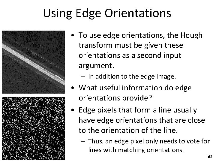
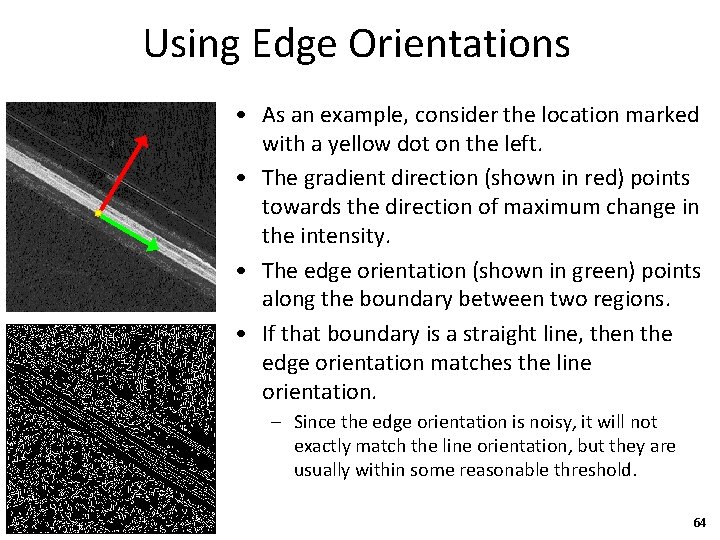
Using Edge Orientations • To use edge orientations, the Hough transform must be given these orientations as a second input argument. – In addition to the edge image. • What useful information do edge orientations provide? • Edge pixels that form a line usually have edge orientations that are close to the orientation of the line. – Thus, an edge pixel only needs to vote for lines with matching orientations. 63

Using Edge Orientations • As an example, consider the location marked with a yellow dot on the left. • The gradient direction (shown in red) points towards the direction of maximum change in the intensity. • The edge orientation (shown in green) points along the boundary between two regions. • If that boundary is a straight line, then the edge orientation matches the line orientation. – Since the edge orientation is noisy, it will not exactly match the line orientation, but they are usually within some reasonable threshold. 64

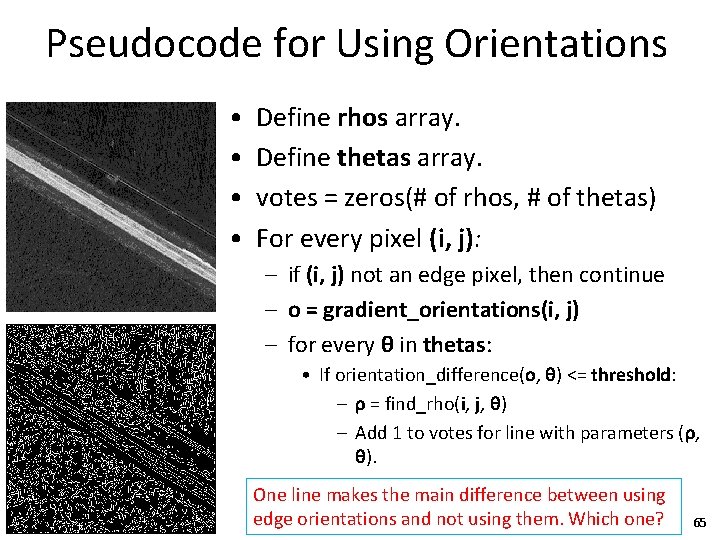
Pseudocode for Using Orientations • • Define rhos array. Define thetas array. votes = zeros(# of rhos, # of thetas) For every pixel (i, j): – if (i, j) not an edge pixel, then continue – o = gradient_orientations(i, j) – for every θ in thetas: • If orientation_difference(ο, θ) <= threshold: – ρ = find_rho(i, j, θ) – Add 1 to votes for line with parameters (ρ, θ). One line makes the main difference between using edge orientations and not using them. Which one? 65

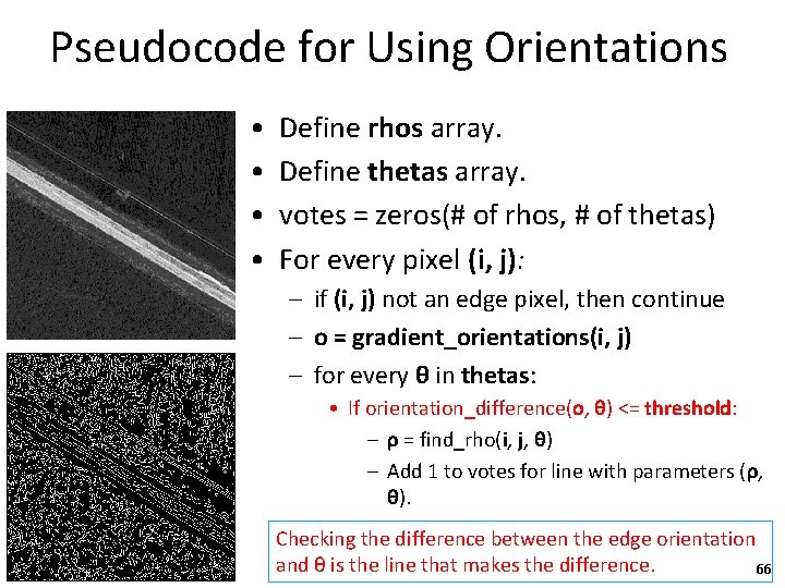
Pseudocode for Using Orientations • • Define rhos array. Define thetas array. votes = zeros(# of rhos, # of thetas) For every pixel (i, j): – if (i, j) not an edge pixel, then continue – o = gradient_orientations(i, j) – for every θ in thetas: • If orientation_difference(ο, θ) <= threshold: – ρ = find_rho(i, j, θ) – Add 1 to votes for line with parameters (ρ, θ). Checking the difference between the edge orientation and θ is the line that makes the difference. 66

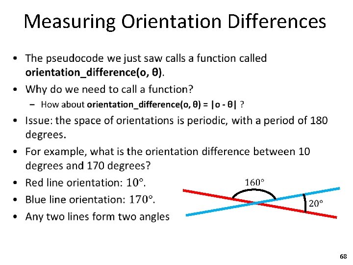
Measuring Orientation Differences • The pseudocode we just saw calls a function called orientation_difference(ο, θ). • Why do we need to call a function? – How about orientation_difference(ο, θ) = |o - θ| ? 67

Measuring Orientation Differences • 68

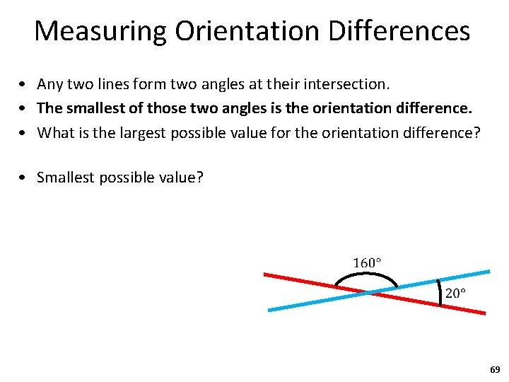
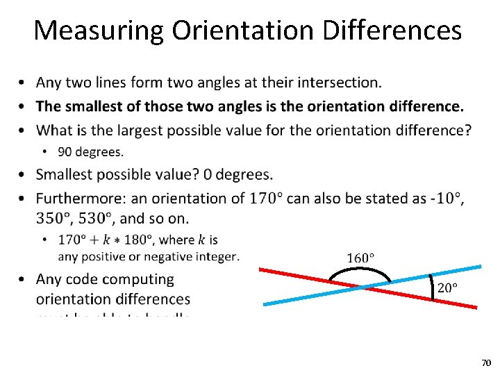
Measuring Orientation Differences • Any two lines form two angles at their intersection. • The smallest of those two angles is the orientation difference. • What is the largest possible value for the orientation difference? • Smallest possible value? 69

Measuring Orientation Differences • 70

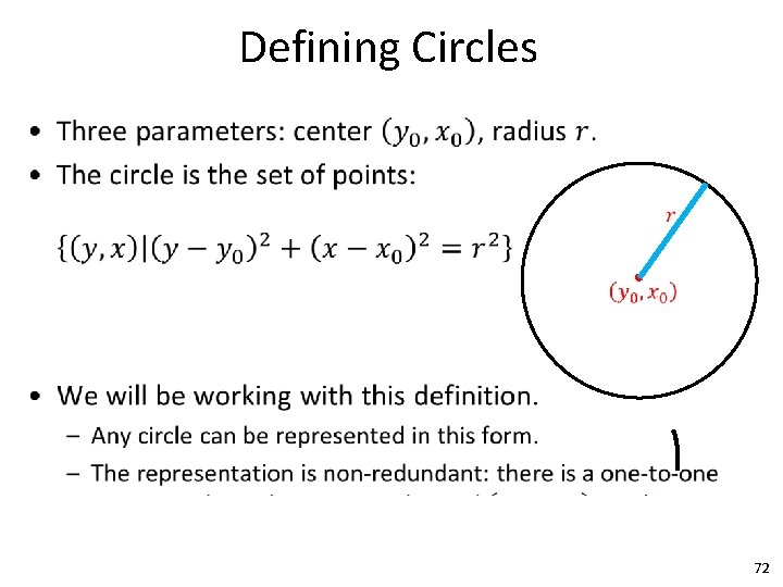
Hough Transform for Circles • There is also a Hough Transform for detecting circles. • The steps for defining and implementing this variant are similar to the ones we took for finding lines. – Find a representation of circles that is convenient to use. – Discretize the infinite set of circles to a finite set. – Every edge pixel votes for all the circles (from the discretized, finite set) that it could belong to. • As for lines, we can optionally use edge orientations to vote for a more restricted set of circles. 71

Defining Circles • 72

Hough Transform on Circles • What is the voting space? • Who votes? • What does each voter vote for? 73

Hough Transform on Circles • What is the voting space? – A discretized version of the set of all circles that can be defined. – size of array: • Who votes? • What does each voter vote for? 74

Hough Transform on Circles • What is the voting space? – A discretized version of the set of all circles that can be defined. – size of array: # centers * # radii. – We get to choose the level of discretization. • Who votes? • What does each voter vote for? 75

Hough Transform on Circles • What is the voting space? – A discretized version of the set of all circles that can be defined. • Who votes? – Every edge pixel. • What does each voter vote for? 76

Hough Transform on Circles • What is the voting space? – A discretized version of the set of all circles that can be defined. • Who votes? – Every edge pixel. • What does each voter vote for? – Every edge pixel votes for all the circles that it belongs to. 77

Hough Transform on Circles • What is the voting space? – A discretized version of the set of all circles that can be defined. • Who votes? – Every edge pixel. • What does each voter vote for? – Every edge pixel votes for all the circles that it belongs to. – Faster version: 78

Hough Transform on Circles • What is the voting space? – A discretized version of the set of all circles that can be defined. • Who votes? – Every edge pixel. • What does each voter vote for? – Every edge pixel votes for all the circles that it belongs to. – Faster version: each edge pixel (i, j) only votes for circles that it can belong to, AND such that the line from (i, j) to the circle center makes a relatively small angle with the gradient orientation at (i, j). 79

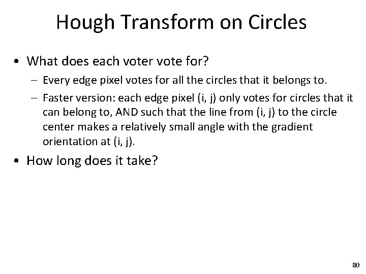
Hough Transform on Circles • What does each voter vote for? – Every edge pixel votes for all the circles that it belongs to. – Faster version: each edge pixel (i, j) only votes for circles that it can belong to, AND such that the line from (i, j) to the circle center makes a relatively small angle with the gradient orientation at (i, j). • How long does it take? 80

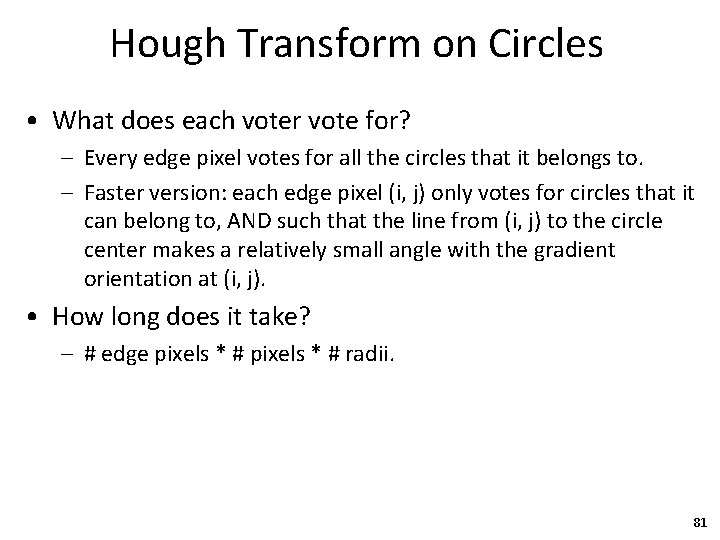
Hough Transform on Circles • What does each voter vote for? – Every edge pixel votes for all the circles that it belongs to. – Faster version: each edge pixel (i, j) only votes for circles that it can belong to, AND such that the line from (i, j) to the circle center makes a relatively small angle with the gradient orientation at (i, j). • How long does it take? – # edge pixels * # radii. 81

General Hough Transforms • In theory, we can use Hough transforms to detect more complicated shapes. • In practice, this requires memory and time exponential to the number of parameters, and is usually not practical. 82